49. Equilibrium Capital Structures with Incomplete Markets#
In addition to what’s in Anaconda, this lecture will need the following libraries:
!pip install --upgrade quantecon
!conda install -y -c plotly plotly plotly-orca
49.1. Introduction#
This is an extension of an earlier lecture Irrelevance of Capital Structure with Complete Markets about a complete markets model.
In contrast to that lecture, this one describes an instance of a model authored by Bisin, Clementi, and Gottardi [Bisin et al., 2018] in which financial markets are incomplete.
Instead of being able to trade equities and a full set of one-period Arrow securities as they can in Irrelevance of Capital Structure with Complete Markets, here consumers and firms trade only equity and a bond.
It is useful to watch how outcomes differ in the two settings.
In the complete markets economy in Irrelevance of Capital Structure with Complete Markets
there is a unique stochastic discount factor that prices all assets
consumers’ portfolio choices are indeterminate
firms’ financial structures are indeterminate, so the model embodies an instance of a Modigliani-Miller irrelevance theorem [Modigliani and Miller, 1958]
the aggregate of all firms’ financial structures are indeterminate, a consequence of there being redundant assets
In the incomplete markets economy studied here
there is a not a unique equilibrium stochastic discount factor
different stochastic discount factors price different assets
consumers’ portfolio choices are determinate
while individual firms’ financial structures are indeterminate, thus conforming to part of a Modigliani-Miller theorem, [Modigliani and Miller, 1958], the aggregate of all firms’ financial structures is determinate.
A Big K, little k analysis played an important role in the previous lecture Irrelevance of Capital Structure with Complete Markets.
A more subtle version of a Big K, little k features in the BCG incomplete markets environment here.
We use it to convey the heart of what BCG call a rational conjectures equilibrium in which conjectures are about equilibrium pricing functions in regions of the state space that an average consumer or firm does not visit in equilibrium.
Note that the absence of complete markets means that now we cannot compute competitive equilibrium prices and allocations by first solving the simple planning problem that we did in Irrelevance of Capital Structure with Complete Markets.
Instead, we compute an equilibrium by solving a system of simultaneous inequalities.
(Here we do not address the interesting question of whether there is a different planning problem that we could use to compute a competitive equlibrium allocation.)
49.1.1. Setup#
We adopt specifications of preferences and technologies used by Bisin, Clemente, and Gottardi (2018) [Bisin et al., 2018] and in our earlier lecture on a complete markets version of their model.
The economy lasts for two periods, \(t=0, 1\).
There are two types of consumers named \(i=1,2\).
A scalar random variable \(\epsilon\) affects both
a representative firm’s physical return \(f(k)e^\epsilon\) in period \(1\) from investing \(k \geq 0\) in capital in period \(0\).
period \(1\) endowments \(w_1^i(\epsilon)\) of the consumption good for agents \(i =1\) and \(i=2\).
49.1.2. Ownership#
A consumer of type \(i\) is endowed with \(w_0^i\) units of the time \(0\) good and \(w_1^i(\epsilon)\) of the time \(1\) good when the random variable takes value \(\epsilon\).
At the start of period \(0\), a consumer of type \(i\) also owns \(\theta^i_0\) shares of a representative firm.
49.1.3. Measures of agents and firms#
As in the companion lecture Irrelevance of Capital Structure with Complete Markets that studies a complete markets version of the model, we follow BCG in assuming that there are unit measures of
consumers of type \(i=1\)
consumers of type \(i=2\)
firms with access to a production technology that converts \(k\) units of time \(0\) good into \(A k^\alpha e^\epsilon\) units of the time \(1\) good in random state \(\epsilon\)
Thus, let \(\omega \in [0,1]\) index a particular consumer of type \(i\).
Then define Big \(C^i\) as
with components
In the same spirit, let \(\zeta \in [0,1]\) index a particular firm and let firm \(\zeta\) purchase \(k(\zeta)\) units of capital and issue \(b(\zeta)\) bonds.
Then define Big \(K\) and Big \(B\) as
The assumption that there are equal measures of our three types of agents justifies our assumption that each individual agent is a powerless price taker:
an individual consumer chooses its own (infinitesimal) part \(c^i(\omega)\) of \(C^i\) taking prices as given
an individual firm chooses its own (infinitesmimal) part \(k(\zeta)\) of \(K\) and \(b(\zeta)\) of \(B\) taking pricing functions as given
However, equilibrium prices depend on the
Big K, Big B, Big Cobjects \(K\), \(B\), and \(C\)
The assumption about measures of agents is a powerful device for making a host of competitive agents take as given the equilibrium prices that turn out to be determined by the decisions of hosts of agents who are just like them.
We call an equilibrium symmetric if
all type \(i\) consumers choose the same consumption profiles so that \(c^i(\omega) = C^i\) for all \(\omega \in [0,1]\)
all firms choose the same levels of \(k\) and \(b\) so that \(k(\zeta) = K\), \(b(\zeta) = B\) for all \(\zeta \in [0,1]\)
In this lecture, we restrict ourselves to describing symmetric equilibria.
49.1.4. Endowments#
Per capital economy-wide endowments in periods \(0\) and \(1\) are
49.1.5. Feasibility:#
Where \(\alpha \in (0,1)\) and \(A >0\)
where \(f(k) = A k^\alpha, A >0, \alpha \in (0,1)\).
49.1.6. Parameterizations#
Following BCG, we shall employ the following parameterizations:
Sometimes instead of asuming \(\epsilon \sim g(\epsilon) = {\mathcal N}(0,\sigma^2)\), we’ll assume that \(g(\cdot)\) is a probability mass function that serves as a discrete approximation to a standardized normal density.
49.1.7. Preferences:#
A consumer of type \(i\) orders period \(0\) consumption \(c_0^i\) and state \(\epsilon\)-period \(1\) consumption \(c^i(\epsilon)\) by
\(\beta \in (0,1)\) and the one-period utility function is
49.1.8. Risk-sharing motives#
The two types of agents’ period \(1\) endowments have different correlations with the physical return on capital.
Endowment differences give agents incentives to trade risks that in the complete market version of the model showed up in their demands for equity and in their demands and supplies of one-period Arrow securities.
In the incomplete-markets setting under study here, these differences show up in differences in the two types of consumers’ demands for a typical firm’s bonds and equity, the only two assets that agents can now trade.
49.2. Asset markets#
Markets are incomplete: ex cathedra we the model builders declare that only equities and bonds issued by representative firms can be traded.
Let \(\theta^i\) and \(\xi^i\) be a consumer of type \(i\)’s post-trade holdings of equity and bonds, respectively.
A firm issues bonds promising to pay \(b\) units of consumption at time \(t=1\) and purchases \(k\) units of physical capital at time \(t=0\).
When \(e^\epsilon A k^\alpha < b\) at time \(1\), the firm defaults and its output is divided equally among bondholders.
Evidently, when the productivity shock \(\epsilon < \epsilon^* = \log \left(\frac{b}{ Ak^\alpha}\right)\), the firm defaults on its debt
Payoffs to equity and debt at date 1 as functions of the productivity shock \(\epsilon\) are thus
A firm faces a bond price function \(p(k,b)\) when it issues \(b\) bonds and purchases \(k\) units of physical capital.
A firm’s equity is worth \(q(k,b)\) when it issues \(b\) bonds and purchases \(k\) units of physical capital.
A firm regards an equity-pricing function \(q(k,b)\) and a bond pricing function \(p(k,b)\) as exogenous in the sense that they are not affected by its choices of \(k\) and \(b\).
Consumers face equilibrium prices \(\check q\) and \(\check p\) for bonds and equities, where \(\check q\) and \(\check p\) are both scalars.
Consumers are price takers and only need to know the scalars \(\check q, \check p\).
Firms are price function takers and must know the functions \(q(k,b), p(k,b)\) in order completely to pose their optimum problems.
49.2.1. Consumers#
Each consumer of type \(i\) is endowed with \(w_0^i\) of the time \(0\) consumption good, \(w_1^i(\epsilon)\) of the time \(1\), state \(\epsilon\) consumption good and also owns a fraction \(\theta^i_0 \in (0,1)\) of the initial value of a representative firm, where \(\theta^1_0 + \theta^2_0 = 1\).
The initial value of a representative firm is \(V\) (an object to be determined in a rational expectations equilibrium).
Consumer \(i\) buys \(\theta^i\) shares of equity and buys bonds worth \(\check p \xi^i\) where \(\check p\) is the bond price.
Being a price-taker, a consumer takes \(V\), \(\check q\), \(\check p\), and \(K, B\) as given.
Consumers know that equilibrium payoff functions for bonds and equities take the form
Consumer \(i\)’s optimization problem is
The last two inequalities impose that the consumer cannot short sell either equity or bonds.
In a rational expectations equilibrium, \(\check q = q(K,B)\) and \(\check p = p(K,B)\)
We form consumer \(i\)’s Lagrangian:
Consumer \(i\)’s first-order necessary conditions for an optimum include:
We can combine and rearrange consumer \(i\)’s first-order conditions to become:
These inequalities imply that in a symmetric rational expectations equilibrium consumption allocations and prices satisfy
49.2.2. Pricing functions#
When individual firms solve their optimization problems, they take big \(C^i\)’s as fixed objects that they don’t influence.
A representative firm faces a price function \(q(k,b)\) for its equity and a price function \(p(k, b)\) per unit of bonds that satisfy
where the payoff functions are described by equations (49.1).
Notice the appearance of big \(C^i\)’s on the right sides of these two equations that define equilibrium pricing functions.
The two price functions describe outcomes not only for equilibrium choices \(K, B\) of capital \(k\) and debt \(b\), but also for any out-of-equilibrium pairs \((k, b) \neq (K, B)\).
The firm is assumed to know both price functions.
This means that the firm understands that its choice of \(k,b\) influences how markets price its equity and debt.
This package of assumptions is sometimes called rational conjectures (about price functions).
BCG give credit to Makowski for emphasizing and clarifying how rational conjectures are components of rational expectations equilibria.
49.2.3. Firms#
The firm chooses capital \(k\) and debt \(b\) to maximize its market value:
Attributing value maximization to the firm is a good idea because in equilibrium consumers of both types want a firm to maximize its value.
In the special quantitative examples studied here
consumers of types \(i=1,2\) both hold equity
only consumers of type \(i=2\) hold debt; consumers of type \(i=1\) hold none.
These outcomes occur because we follow BCG and set parameters so that a type 2 consumer’s stochastic endowment of the consumption good in period \(1\) is more correlated with the firm’s output than is a type 1 consumer’s.
This gives consumers of type \(2\) a motive to hedge their second period endowment risk by holding bonds (they also choose to hold some equity).
These outcomes mean that the pricing functions end up satisfying
Recall that \(\epsilon^*(k,b) \equiv \log\left(\frac{b}{Ak^\alpha}\right)\) is a firm’s default threshold.
We can rewrite the pricing functions as:
49.2.3.1. Firm’s optimization problem#
The firm’s optimization problem is
The firm’s first-order necessary conditions with respect to \(k\) and \(b\), respectively, are
We use the Leibniz integral rule several times to arrive at the following derivatives:
Special case: We confine ourselves to a special case in which both types of consumer hold positive equities so that \(\frac{\partial q(k,b)}{\partial k}\) and \(\frac{\partial q(k,b)}{\partial b}\) are related to rates of intertemporal substitution for both agents.
Substituting these partial derivatives into the above first-order conditions for \(k\) and \(b\), respectively, we obtain the following versions of those first order conditions:
where again recall that \(\epsilon^*(k,b) \equiv \log\left(\frac{b}{Ak^\alpha}\right)\).
Taking \(C_0^i, C_1^i(\epsilon)\) as given, these are two equations that we want to solve for the firm’s optimal decisions \(k, b\).
49.3. Equilibrium verification#
On page 5 of BCG (2018), the authors say
If the price conjectures corresponding to the plan chosen by firms in equilibrium are correct, that is equal to the market prices \(\check q\) and \(\check p\), it is immediate to verify that the rationality of the conjecture coincides with the agents’ Euler equations.
Here BCG are describing how they go about verifying that when they set little \(k\), little \(b\) from the firm’s first-order conditions equal to the big \(K\), big \(B\) at the big \(C\)’s that appear in the pricing functions, then
consumers’ Euler equations are satisfied if little \(c\)’s are equated to Big \(C\)’s
firms’ first-order necessary conditions for \(k, b\) are satisfied.
\(\check q = q(K,B)\) and \(\check p = p(K,B)\).
49.4. Pseudo code#
Before displaying our Python code for computing a BCG incomplete markets equilibrium, we’ll sketch some pseudo code that describes its logical flow.
Here goes:
Set upper and lower bounds for firm value as \(V_h\) and \(V_l\), for capital as \(k_h\) and \(k_l\), and for debt as \(b_h\) and \(b_l\).
Conjecture firm value \(V = \frac{1}{2}(V_h + V_l)\)
Conjecture debt level \(b = \frac{1}{2}(b_h + b_l)\).
Conjecture capital \(k = \frac{1}{2}(k_h + k_l)\).
Compute the default threshold \(\epsilon^* \equiv \log\left(\frac{b}{Ak^\alpha}\right)\).
(In this step we abuse notation by freezing \(V, k, b\) and in effect temporarily treating them as Big \(K,B\) values. Thus, in this step 6 little \(k, b\) are frozen at guessed at value of \(K, B\).) Fixing the values of \(V\), \(b\) and \(k\), compute optimal choices of consumption \(c^i\) with consumers’ FOCs. Assume that only agent 2 holds debt: \(\xi^2 = b\) and that both agents hold equity: \(0 <\theta^i < 1\) for \(i=1,2\).
Set high and low bounds for equity holdings for agent 1 as \(\theta^1_h\) and \(\theta^1_l\). Guess \(\theta^1 = \frac{1}{2}(\theta^1_h + \theta^1_l)\), and \(\theta^2 = 1 - \theta^1\). While \(|\theta^1_h - \theta^1_l|\) is large:
Compute agent 1’s valuation of the equity claim with a fixed-point iteration:
\(q_1 = \beta \int \frac{u^\prime(c^1_1(\epsilon))}{u^\prime(c^1_0)} d^e(k,b;\epsilon) g(\epsilon) \ d\epsilon\)
where
\(c^1_1(\epsilon) = w^1_1(\epsilon) + \theta^1 d^e(k,b;\epsilon)\)
and
\(c^1_0 = w^1_0 + \theta^1_0V - q_1\theta^1\)
Compute agent 2’s valuation of the bond claim with a fixed-point iteration:
\(p = \beta \int \frac{u^\prime(c^2_1(\epsilon))}{u^\prime(c^2_0)} d^b(k,b;\epsilon) g(\epsilon) \ d\epsilon\)
where
\(c^2_1(\epsilon) = w^2_1(\epsilon) + \theta^2 d^e(k,b;\epsilon) + b\)
and
\(c^2_0 = w^2_0 + \theta^2_0 V - q_1 \theta^2 - pb\)
Compute agent 2’s valuation of the equity claim with a fixed-point iteration:
\(q_2 = \beta \int \frac{u^\prime(c^2_1(\epsilon))}{u^\prime(c^2_0)} d^e(k,b;\epsilon) g(\epsilon) \ d\epsilon\)
where
\(c^2_1(\epsilon) = w^2_1(\epsilon) + \theta^2 d^e(k,b;\epsilon) + b\)
and
\(c^2_0 = w^2_0 + \theta^2_0 V - q_2 \theta^2 - pb\)
If \(q_1 > q_2\), Set \(\theta_l = \theta^1\); otherwise, set \(\theta_h = \theta^1\).
Repeat steps 6Aa through 6Ad until \(|\theta^1_h - \theta^1_l|\) is small.
Set bond price as \(p\) and equity price as \(q = \max(q_1,q_2)\).
Compute optimal choices of consumption:
\[\begin{split} \begin{aligned} c^1_0 &= w^1_0 + \theta^1_0V - q\theta^1 \\ c^2_0 &= w^2_0 + \theta^2_0V - q\theta^2 - pb \\ c^1_1(\epsilon) &= w^1_1(\epsilon) + \theta^1 d^e(k,b;\epsilon) \\ c^2_1(\epsilon) &= w^2_1(\epsilon) + \theta^2 d^e(k,b;\epsilon) + b \end{aligned} \end{split}\](Here we confess to abusing notation again, but now in a different way. In step 7, we interpret frozen \(c^i\)s as Big \(C^i\). We do this to solve the firm’s problem.) Fixing the values of \(c^i_0\) and \(c^i_1(\epsilon)\), compute optimal choices of capital \(k\) and debt level \(b\) using the firm’s first order necessary conditions.
Compute deviations from the firm’s FONC for capital \(k\) as:
\(kfoc = \beta \alpha A k^{\alpha - 1} \left( \int \frac{u^\prime(c^2_1(\epsilon))}{u^\prime(c^2_0)} e^\epsilon g(\epsilon) \ d\epsilon \right) - 1\)
If \(kfoc > 0\), Set \(k_l = k\); otherwise, set \(k_h = k\).
Repeat steps 4 through 7A until \(|k_h-k_l|\) is small.
Compute deviations from the firm’s FONC for debt level \(b\) as:
\(bfoc = \beta \left[ \int_{\epsilon^*}^\infty \left( \frac{u^\prime(c^1_1(\epsilon))}{u^\prime(c^1_0)} \right) g(\epsilon) \ d\epsilon - \int_{\epsilon^*}^\infty \left( \frac{u^\prime(c^2_1(\epsilon))}{u^\prime(c^2_0)} \right) g(\epsilon) \ d\epsilon \right]\)
If \(bfoc > 0\), Set \(b_h = b\); otherwise, set \(b_l = b\).
Repeat steps 3 through 7B until \(|b_h-b_l|\) is small.
Given prices \(q\) and \(p\) from step 6, and the firm choices of \(k\) and \(b\) from step 7, compute the synthetic firm value:
\(V_x = -k + q + pb\)
If \(V_x > V\), then set \(V_l = V\); otherwise, set \(V_h = V\).
Repeat steps 1 through 8 until \(|V_x - V|\) is small.
Ultimately, the algorithm returns equilibrium capital \(k^*\), debt \(b^*\) and firm value \(V^*\), as well as the following equilibrium values:
Equity holdings \(\theta^{1,*} = \theta^1(k^*,b^*)\)
Prices \(q^*=q(k^*,b^*), \ p^*=p(k^*,b^*)\)
Consumption plans \(C^{1,*}_0 = c^1_0(k^*,b^*),\ C^{2,*}_0 = c^2_0(k^*,b^*), \ C^{1,*}_1(\epsilon) = c^1_1(k^*,b^*;\epsilon),\ C^{1,*}_1(\epsilon) = c^2_1(k^*,b^*;\epsilon)\).
49.5. Code#
We create a Python class BCG_incomplete_markets to compute the
equilibrium allocations of the incomplete market BCG model, given a set
of parameter values.
The class includes the following methods, i.e., functions:
solve_eq: solves the BCG model and returns the equilibrium values of capital \(k\), debt \(b\) and firm value \(V\), as well asagent 1’s equity holdings \(\theta^{1,*}\)
prices \(q^*, p^*\)
consumption plans \(C^{1,*}_0, C^{2,*}_0, C^{1,*}_1(\epsilon), C^{2,*}_1(\epsilon)\).
eq_valuation: inputs equilibrium consumpion plans \(C^*\) and outputs the following valuations for each pair of \((k,b)\) in the grid:the firm \(V(k,b)\)
the equity \(q(k,b)\)
the bond \(p(k,b)\).
Parameters include:
\(\chi_1\), \(\chi_2\): correlation parameter for agent 1 and 2. Default values are respectively 0 and 0.9.
\(w^1_0\), \(w^2_0\): initial endowments. Default values are respectively 0.9 and 1.1.
\(\theta^1_0\), \(\theta^2_0\): initial holding of the firm. Default values are 0.5.
\(\psi\): risk parameter. Default value is 3.
\(\alpha\): Production function parameter. Default value is 0.6.
\(A\): Productivity of the firm. Default value is 2.5.
\(\mu\), \(\sigma\): Mean and standard deviation of the shock distribution. Default values are respectively -0.025 and 0.4
\(\beta\): Discount factor. Default value is 0.96.
bound: Bound for truncated normal distribution. Default value is 3.
import numpy as np
from scipy.stats import truncnorm
from scipy.integrate import quad
from numba import njit
class BCG_incomplete_markets:
# init method or constructor
def __init__(self,
𝜒1 = 0,
𝜒2 = 0.9,
w10 = 0.9,
w20 = 1.1,
𝜃10 = 0.5,
𝜃20 = 0.5,
𝜓1 = 3,
𝜓2 = 3,
𝛼 = 0.6,
A = 2.5,
𝜇 = -0.025,
𝜎 = 0.4,
𝛽 = 0.96,
bound = 3,
Vl = 0,
Vh = 0.5,
kbot = 0.01,
#ktop = (𝛼*A)**(1/(1-𝛼)),
ktop = 0.25,
bbot = 0.1,
btop = 0.8):
#=========== Setup ===========#
# Risk parameters
self.𝜒1 = 𝜒1
self.𝜒2 = 𝜒2
# Other parameters
self.𝜓1 = 𝜓1
self.𝜓2 = 𝜓2
self.𝛼 = 𝛼
self.A = A
self.𝜇 = 𝜇
self.𝜎 = 𝜎
self.𝛽 = 𝛽
self.bound = bound
# Bounds for firm value, capital, and debt
self.Vl = Vl
self.Vh = Vh
self.kbot = kbot
#self.kbot = (𝛼*A)**(1/(1-𝛼))
self.ktop = ktop
self.bbot = bbot
self.btop = btop
# Utility
self.u = njit(lambda c: (c**(1-𝜓)) / (1-𝜓))
# Initial endowments
self.w10 = w10
self.w20 = w20
self.w0 = w10 + w20
# Initial holdings
self.𝜃10 = 𝜃10
self.𝜃20 = 𝜃20
# Endowments at t=1
self.w11 = njit(lambda 𝜖: np.exp(-𝜒1*𝜇 - 0.5*(𝜒1**2)*(𝜎**2) + 𝜒1*𝜖))
self.w21 = njit(lambda 𝜖: np.exp(-𝜒2*𝜇 - 0.5*(𝜒2**2)*(𝜎**2) + 𝜒2*𝜖))
self.w1 = njit(lambda 𝜖: self.w11(𝜖) + self.w21(𝜖))
# Truncated normal
ta, tb = (-bound - 𝜇) / 𝜎, (bound - 𝜇) / 𝜎
rv = truncnorm(ta, tb, loc=𝜇, scale=𝜎)
𝜖_range = np.linspace(ta, tb, 1000000)
pdf_range = rv.pdf(𝜖_range)
self.g = njit(lambda 𝜖: np.interp(𝜖, 𝜖_range, pdf_range))
#*************************************************************
# Function: Solve for equilibrium of the BCG model
#*************************************************************
def solve_eq(self, print_crit=True):
# Load parameters
𝜓1 = self.𝜓1
𝜓2 = self.𝜓2
𝛼 = self.𝛼
A = self.A
𝛽 = self.𝛽
bound = self.bound
Vl = self.Vl
Vh = self.Vh
kbot = self.kbot
ktop = self.ktop
bbot = self.bbot
btop = self.btop
w10 = self.w10
w20 = self.w20
𝜃10 = self.𝜃10
𝜃20 = self.𝜃20
w11 = self.w11
w21 = self.w21
g = self.g
# We need to find a fixed point on the value of the firm
V_crit = 1
Y = njit(lambda 𝜖, fk: np.exp(𝜖)*fk)
intqq1 = njit(lambda 𝜖, fk, 𝜃1, 𝜓1, b: (w11(𝜖) + 𝜃1*(Y(𝜖, fk) - b))**(-𝜓1)*(Y(𝜖, fk) - b)*g(𝜖))
intp1 = njit(lambda 𝜖, fk, 𝜓2, b: (Y(𝜖, fk)/b)*(w21(𝜖) + Y(𝜖, fk))**(-𝜓2)*g(𝜖))
intp2 = njit(lambda 𝜖, fk, 𝜃2, 𝜓2, b: (w21(𝜖) + 𝜃2*(Y(𝜖, fk)-b) + b)**(-𝜓2)*g(𝜖))
intqq2 = njit(lambda 𝜖, fk, 𝜃2, 𝜓2, b: (w21(𝜖) + 𝜃2*(Y(𝜖, fk)-b) + b)**(-𝜓2)*(Y(𝜖, fk) - b)*g(𝜖))
intk1 = njit(lambda 𝜖, fk, 𝜓2: (w21(𝜖) + Y(𝜖, fk))**(-𝜓2)*np.exp(𝜖)*g(𝜖))
intk2 = njit(lambda 𝜖, fk, 𝜃2, 𝜓2, b: (w21(𝜖) + 𝜃2*(Y(𝜖, fk)-b) + b)**(-𝜓2)*np.exp(𝜖)*g(𝜖))
intB1 = njit(lambda 𝜖, fk, 𝜃1, 𝜓1, b: (w11(𝜖) + 𝜃1*(Y(𝜖, fk) - b))**(-𝜓1)*g(𝜖))
intB2 = njit(lambda 𝜖, fk, 𝜃2, 𝜓2, b: (w21(𝜖) + 𝜃2*(Y(𝜖, fk) - b) + b)**(-𝜓2)*g(𝜖))
while V_crit>1e-4:
# We begin by adding the guess for the value of the firm to endowment
V = (Vl+Vh)/2
ww10 = w10 + 𝜃10*V
ww20 = w20 + 𝜃20*V
# Figure out the optimal level of debt
bl = bbot
bh = btop
b_crit=1
while b_crit>1e-5:
# Setting the conjecture for debt
b = (bl+bh)/2
# Figure out the optimal level of capital
kl = kbot
kh = ktop
k_crit=1
while k_crit>1e-5:
# Setting the conjecture for capital
k = (kl+kh)/2
# Production
fk = A*(k**𝛼)
# Y = lambda 𝜖: np.exp(𝜖)*fk
# Compute integration threshold
epstar = np.log(b/fk)
#**************************************************************
# Compute the prices and allocations consistent with consumers'
# Euler equations
#**************************************************************
# We impose the following:
# Agent 1 buys equity
# Agent 2 buys equity and all debt
# Agents trade such that prices converge
#========
# Agent 1
#========
# Holdings
𝜉1 = 0
𝜃1a = 0.3
𝜃1b = 1
while abs(𝜃1b - 𝜃1a) > 0.001:
𝜃1 = (𝜃1a + 𝜃1b) / 2
# qq1 is the equity price consistent with agent-1 Euler Equation
## Note: Price is in the date-0 budget constraint of the agent
## First, compute the constant term that is not influenced by q
## that is, 𝛽E[u'(c^{1}_{1})d^{e}(k,B)]
# intqq1 = lambda 𝜖: (w11(𝜖) + 𝜃1*(Y(𝜖, fk) - b))**(-𝜓1)*(Y(𝜖, fk) - b)*g(𝜖)
# const_qq1 = 𝛽 * quad(intqq1,epstar,bound)[0]
const_qq1 = 𝛽 * quad(intqq1,epstar,bound, args=(fk, 𝜃1, 𝜓1, b))[0]
## Second, iterate to get the equity price q
qq1l = 0
qq1h = ww10
diff = 1
while diff > 1e-7:
qq1 = (qq1l+qq1h)/2
rhs = const_qq1/((ww10-qq1*𝜃1)**(-𝜓1));
if (rhs > qq1):
qq1l = qq1
else:
qq1h = qq1
diff = abs(qq1l-qq1h)
#========
# Agent 2
#========
𝜉2 = b - 𝜉1
𝜃2 = 1 - 𝜃1
# p is the bond price consistent with agent-2 Euler Equation
## Note: Price is in the date-0 budget constraint of the agent
## First, compute the constant term that is not influenced by p
## that is, 𝛽E[u'(c^{2}_{1})d^{b}(k,B)]
# intp1 = lambda 𝜖: (Y(𝜖, fk)/b)*(w21(𝜖) + Y(𝜖, fk))**(-𝜓2)*g(𝜖)
# intp2 = lambda 𝜖: (w21(𝜖) + 𝜃2*(Y(𝜖, fk)-b) + b)**(-𝜓2)*g(𝜖)
# const_p = 𝛽 * (quad(intp1,-bound,epstar)[0] + quad(intp2,epstar,bound)[0])
const_p = 𝛽 * (quad(intp1,-bound,epstar, args=(fk, 𝜓2, b))[0]\
+ quad(intp2,epstar,bound, args=(fk, 𝜃2, 𝜓2, b))[0])
## iterate to get the bond price p
pl = 0
ph = ww20/b
diff = 1
while diff > 1e-7:
p = (pl+ph)/2
rhs = const_p/((ww20-qq1*𝜃2-p*b)**(-𝜓2))
if (rhs > p):
pl = p
else:
ph = p
diff = abs(pl-ph)
# qq2 is the equity price consistent with agent-2 Euler Equation
# intqq2 = lambda 𝜖: (w21(𝜖) + 𝜃2*(Y(𝜖, fk)-b) + b)**(-𝜓2)*(Y(𝜖, fk) - b)*g(𝜖)
const_qq2 = 𝛽 * quad(intqq2,epstar,bound, args=(fk, 𝜃2, 𝜓2, b))[0]
qq2l = 0
qq2h = ww20
diff = 1
while diff > 1e-7:
qq2 = (qq2l+qq2h)/2
rhs = const_qq2/((ww20-qq2*𝜃2-p*b)**(-𝜓2));
if (rhs > qq2):
qq2l = qq2
else:
qq2h = qq2
diff = abs(qq2l-qq2h)
# q be the maximum valuation for the equity among agents
## This will be the equity price based on Makowski's criterion
q = max(qq1,qq2)
#================
# Update holdings
#================
if qq1 > qq2:
𝜃1a = 𝜃1
else:
𝜃1b = 𝜃1
#================
# Get consumption
#================
c10 = ww10 - q*𝜃1
c11 = lambda 𝜖: w11(𝜖) + 𝜃1*max(Y(𝜖, fk)-b,0)
c20 = ww20 - q*(1-𝜃1) - p*b
c21 = lambda 𝜖: w21(𝜖) + (1-𝜃1)*max(Y(𝜖, fk)-b,0) + min(Y(𝜖, fk),b)
#*************************************************
# Compute the first order conditions for the firm
#*************************************************
#===========
# Equity FOC
#===========
# Only agent 2's IMRS is relevent
# intk1 = lambda 𝜖: (w21(𝜖) + Y(𝜖, fk))**(-𝜓2)*np.exp(𝜖)*g(𝜖)
# intk2 = lambda 𝜖: (w21(𝜖) + 𝜃2*(Y(𝜖, fk)-b) + b)**(-𝜓2)*np.exp(𝜖)*g(𝜖)
# kfoc_num = quad(intk1,-bound,epstar)[0] + quad(intk2,epstar,bound)[0]
kfoc_num = quad(intk1,-bound,epstar, args=(fk, 𝜓2))[0] + quad(intk2,epstar,bound, args=(fk, 𝜃2, 𝜓2, b))[0]
kfoc_denom = (ww20- q*𝜃2 - p*b)**(-𝜓2)
kfoc = 𝛽*𝛼*A*(k**(𝛼-1))*(kfoc_num/kfoc_denom) - 1
if (kfoc > 0):
kl = k
else:
kh = k
k_crit = abs(kh-kl)
if print_crit:
print("critical value of k: {:.5f}".format(k_crit))
#=========
# Bond FOC
#=========
# intB1 = lambda 𝜖: (w11(𝜖) + 𝜃1*(Y(𝜖, fk) - b))**(-𝜓1)*g(𝜖)
# intB2 = lambda 𝜖: (w21(𝜖) + 𝜃2*(Y(𝜖, fk) - b) + b)**(-𝜓2)*g(𝜖)
# bfoc1 = quad(intB1,epstar,bound)[0] / (ww10 - q*𝜃1)**(-𝜓1)
# bfoc2 = quad(intB2,epstar,bound)[0] / (ww20 - q*𝜃2 - p*b)**(-𝜓2)
bfoc1 = quad(intB1,epstar,bound, args=(fk, 𝜃1, 𝜓1, b))[0] / (ww10 - q*𝜃1)**(-𝜓1)
bfoc2 = quad(intB2,epstar,bound, args=(fk, 𝜃2, 𝜓2, b))[0] / (ww20 - q*𝜃2 - p*b)**(-𝜓2)
bfoc = bfoc1 - bfoc2
if (bfoc > 0):
bh = b
else:
bl = b
b_crit = abs(bh-bl)
if print_crit:
print("#=== critical value of b: {:.5f}".format(b_crit))
# Compute the value of the firm
value_x = -k + q + p*b
if (value_x > V):
Vl = V
else:
Vh = V
V_crit = abs(value_x-V)
if print_crit:
print("#====== critical value of V: {:.5f}".format(V_crit))
print('k,b,p,q,kfoc,bfoc,epstar,V,V_crit')
formattedList = ["%.3f" % member for member in [k,
b,
p,
q,
kfoc,
bfoc,
epstar,
V,
V_crit]]
print(formattedList)
#*********************************
# Equilibrium values
#*********************************
# Return the results
kss = k
bss = b
Vss = V
qss = q
pss = p
c10ss = c10
c11ss = c11
c20ss = c20
c21ss = c21
𝜃1ss = 𝜃1
# Print the results
print('finished')
# print('k,b,p,q,kfoc,bfoc,epstar,V,V_crit')
#formattedList = ["%.3f" % member for member in [kss,
# bss,
# pss,
# qss,
# kfoc,
# bfoc,
# epstar,
# Vss,
# V_crit]]
#print(formattedList)
return kss,bss,Vss,qss,pss,c10ss,c11ss,c20ss,c21ss,𝜃1ss
#*************************************************************
# Function: Equity and bond valuations by different agents
#*************************************************************
def valuations_by_agent(self,
c10, c11, c20, c21,
k, b):
# Load parameters
𝜓1 = self.𝜓1
𝜓2 = self.𝜓2
𝛼 = self.𝛼
A = self.A
𝛽 = self.𝛽
bound = self.bound
Vl = self.Vl
Vh = self.Vh
kbot = self.kbot
ktop = self.ktop
bbot = self.bbot
btop = self.btop
w10 = self.w10
w20 = self.w20
𝜃10 = self.𝜃10
𝜃20 = self.𝜃20
w11 = self.w11
w21 = self.w21
g = self.g
# Get functions for IMRS/state price density
IMRS1 = lambda 𝜖: 𝛽 * (c11(𝜖)/c10)**(-𝜓1)*g(𝜖)
IMRS2 = lambda 𝜖: 𝛽 * (c21(𝜖)/c20)**(-𝜓2)*g(𝜖)
# Production
fk = A*(k**𝛼)
Y = lambda 𝜖: np.exp(𝜖)*fk
# Compute integration threshold
epstar = np.log(b/fk)
# Compute equity valuation with agent 1's IMRS
intQ1 = lambda 𝜖: IMRS1(𝜖)*(Y(𝜖) - b)
Q1 = quad(intQ1, epstar, bound)[0]
# Compute bond valuation with agent 1's IMRS
intP1 = lambda 𝜖: IMRS1(𝜖)*Y(𝜖)/b
P1 = quad(intP1, -bound, epstar)[0] + quad(IMRS1, epstar, bound)[0]
# Compute equity valuation with agent 2's IMRS
intQ2 = lambda 𝜖: IMRS2(𝜖)*(Y(𝜖) - b)
Q2 = quad(intQ2, epstar, bound)[0]
# Compute bond valuation with agent 2's IMRS
intP2 = lambda 𝜖: IMRS2(𝜖)*Y(𝜖)/b
P2 = quad(intP2, -bound, epstar)[0] + quad(IMRS2, epstar, bound)[0]
return Q1,Q2,P1,P2
#*************************************************************
# Function: equilibrium valuations for firm, equity, bond
#*************************************************************
def eq_valuation(self, c10, c11, c20, c21, N=30):
# Load parameters
𝜓1 = self.𝜓1
𝜓2 = self.𝜓2
𝛼 = self.𝛼
A = self.A
𝛽 = self.𝛽
bound = self.bound
Vl = self.Vl
Vh = self.Vh
kbot = self.kbot
ktop = self.ktop
bbot = self.bbot
btop = self.btop
w10 = self.w10
w20 = self.w20
𝜃10 = self.𝜃10
𝜃20 = self.𝜃20
w11 = self.w11
w21 = self.w21
g = self.g
# Create grids
kgrid, bgrid = np.meshgrid(np.linspace(kbot,ktop,N),
np.linspace(bbot,btop,N))
Vgrid = np.zeros_like(kgrid)
Qgrid = np.zeros_like(kgrid)
Pgrid = np.zeros_like(kgrid)
# Loop: firm value
for i in range(N):
for j in range(N):
# Get capital and debt
k = kgrid[i,j]
b = bgrid[i,j]
# Valuations by each agent
Q1,Q2,P1,P2 = self.valuations_by_agent(c10,
c11,
c20,
c21,
k,
b)
# The prices will be the maximum of the valuations
Q = max(Q1,Q2)
P = max(P1,P2)
# Compute firm value
V = -k + Q + P*b
Vgrid[i,j] = V
Qgrid[i,j] = Q
Pgrid[i,j] = P
return kgrid, bgrid, Vgrid, Qgrid, Pgrid
49.6. Examples#
Below we show some examples computed with the class BCG_incomplete markets.
49.6.1. First example#
In the first example, we set up an instance of the BCG incomplete markets model with default parameter values.
mdl = BCG_incomplete_markets()
kss,bss,Vss,qss,pss,c10ss,c11ss,c20ss,c21ss,𝜃1ss = mdl.solve_eq(print_crit=False)
print(-kss+qss+pss*bss)
print(Vss)
print(𝜃1ss)
0.10073912888808995
0.100830078125
0.98564453125
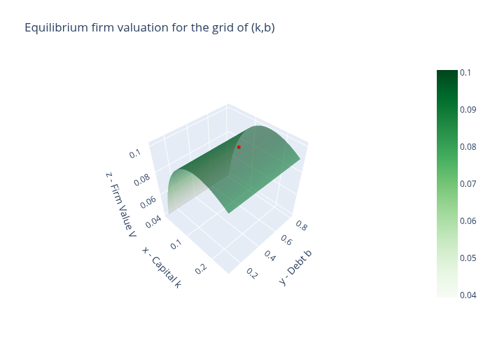
Python reports to us that the equilibrium firm value is \(V=0.101\), with capital \(k = 0.151\) and debt \(b=0.484\).
Let’s verify some things that have to be true if our algorithm has truly found an equilibrium.
Thus, let’s see if the firm is actually maximizing its firm value given the equilibrium pricing function \(q(k,b)\) for equity and \(p(k,b)\) for bonds.
kgrid, bgrid, Vgrid, Qgrid, Pgrid = mdl.eq_valuation(c10ss, c11ss, c20ss, c21ss,N=30)

print('Maximum valuation of the firm value in the (k,B) grid: {:.5f}'.format(Vgrid.max()))
print('Equilibrium firm value: {:.5f}'.format(Vss))
Maximum valuation of the firm value in the (k,B) grid: 0.10074
Equilibrium firm value: 0.10083
Up to the approximation involved in using a discrete grid, these numbers give us comfort that the firm does indeed seem to be maximizing its value at the top of the value hill on the \((k,b)\) plane that it faces.
Below we will plot the firm’s value as a function of \(k,b\).
We’ll also plot the equilibrium price functions \(q(k,b)\) and \(p(k,b)\).
from IPython.display import Image
import matplotlib.pyplot as plt
from mpl_toolkits import mplot3d
import plotly.graph_objs as go

# Firm Valuation
fig = go.Figure(data=[go.Scatter3d(x=[kss],
                                   y=[bss],
                                   z=[Vss],
                                   mode='markers',
                                   marker=dict(size=3, color='red')),
                      go.Surface(x=kgrid,
                                 y=bgrid,
                                 z=Vgrid,
                                 colorscale='Greens',opacity=0.6)])

fig.update_layout(scene = dict(
                    xaxis_title='x - Capital k',
                    yaxis_title='y - Debt b',
                    zaxis_title='z - Firm Value V',
                    aspectratio = dict(x=1,y=1,z=1)),
                  width=700,
                  height=700,
                  margin=dict(l=50, r=50, b=65, t=90))
fig.update_layout(scene_camera=dict(eye=dict(x=1.5, y=-1.5, z=2)))
fig.update_layout(title='Equilibrium firm valuation for the grid of (k,b)')

# Export to PNG file
Image(fig.to_image(format="png", engine="kaleido"))
# fig.show() will provide interactive plot when running
# code locally
/tmp/ipykernel_6296/3275228647.py:29: DeprecationWarning:


Support for the 'engine' argument is deprecated and will be removed after September 2025.
Kaleido will be the only supported engine at that time.
49.6.1.1. A Modigliani-Miller theorem?#
The red dot in the above graph is both an equilibrium \((b,k)\) chosen by a representative firm and the equilibrium \(B, K\) pair chosen by the aggregate of all firms.
Thus, in equilibrium it is true that
But an individual firm named \(\zeta \in [0,1]\) neither knows nor cares whether it sets \((b(\zeta),k(\zeta)) = (B,K)\).
Indeed the above graph has a ridge of \(b(\zeta)\)’s that also maximize the firm’s value so long as it sets \(k(\zeta) = K\).
Here it is important that the measure of firms that deviate from setting \(b\) at the red dot is very small – measure zero – so that \(B\) remains at the red dot even while one firm \(\zeta\) deviates.
So within this equilibrium, there is a qualified Modigliani-Miller theorem that asserts that firm \(\zeta\)’s value is independent of how it mixes its financing between equity and bonds (so long as it is not what other firms do on average).
Thus, while an individual firm \(\zeta\)’s financial structure is indeterminate, the market’s financial structure is determinant and sits at the red dot in the above graph.
This contrasts sharply with the unqualified Modigliani-Miller theorem descibed in the complete markets model in the lecture Irrelevance of Capital Structure with Complete Markets.
There the market’s financial structure was indeterminate.
These subtle distinctions bear more thought and exploration.
So we will do some calculations to ferret out a sense in which the equilibrium \((k,b) = (K,B)\) outcome at the red dot in the above graph is stable.
In particular, we’ll explore the consequences of some choices of \(b=B\) that deviate from the red dot and ask whether firm \(\zeta\) would want to remain at that \(b\).
In more detail, here is what we’ll do:
Obtain equilibrium values of capital and debt as \(k^*=K\) and \(b^*=B\), the red dot above.
Now fix \(k^*\) and let \(b^{**} = b^* - e\) for some \(e > 0\). Conjecture that big \(K = k^*\) but big \(B = b^{**}\).
Take \(K\) and \(B\) and compute intertermporal marginal rates of substitution (IMRS’s) as we did before.
Taking the new IMRS to the firm’s problem. Plot 3D surface for the valuations of the firm with this new IMRS.
Check if the value at \(k^*\), \(b^{**}\) is at the top of this new 3D surface.
Repeat these calculations for \(b^{**} = b^* + e\).
To conduct the above procedures, we create a function off_eq_check
that inputs the BCG model instance parameters, equilibrium capital
\(K=k^*\) and debt \(B=b^*\), and a perturbation of debt \(e\).
The function outputs the fixed point firm values \(V^{**}\), prices \(q^{**}\), \(p^{**}\), and consumption choices \(c^{**}\).
Importantly, we relax the condition that only agent 2 holds bonds.
Now both agents can hold bonds, i.e., \(0\leq \xi^1 \leq B\) and \(\xi^1 +\xi^2 = B\).
That implies the consumers’ budget constraints are:
The function also outputs agent 1’s bond holdings \(\xi_1\).
def off_eq_check(mdl,kss,bss,e=0.1):
    # Big K and big B
    k = kss
    b = bss + e

    # Load parameters
    𝜓1 = mdl.𝜓1
    𝜓2 = mdl.𝜓2
    𝛼 = mdl.𝛼
    A = mdl.A
    𝛽 = mdl.𝛽
    bound = mdl.bound
    Vl = mdl.Vl
    Vh = mdl.Vh
    kbot = mdl.kbot
    ktop = mdl.ktop
    bbot = mdl.bbot
    btop = mdl.btop
    w10 = mdl.w10
    w20 = mdl.w20
    𝜃10 = mdl.𝜃10
    𝜃20 = mdl.𝜃20
    w11 = mdl.w11
    w21 = mdl.w21
    g = mdl.g

    Y = njit(lambda 𝜖, fk: np.exp(𝜖)*fk)
    intqq1 = njit(lambda 𝜖, fk, 𝜃1, 𝜓1, 𝜉1, b: (w11(𝜖) + 𝜃1*(Y(𝜖, fk) - b) + 𝜉1)**(-𝜓1)*(Y(𝜖, fk) - b)*g(𝜖))
    intpp1a = njit(lambda 𝜖, fk, 𝜓1, 𝜉1, b: (Y(𝜖, fk)/b)*(w11(𝜖) + Y(𝜖, fk)/b*𝜉1)**(-𝜓1)*g(𝜖))
    intpp1b = njit(lambda 𝜖, fk, 𝜃1, 𝜓1, 𝜉1, b: (w11(𝜖) + 𝜃1*(Y(𝜖, fk)-b) + 𝜉1)**(-𝜓1)*g(𝜖))
    intpp2a = njit(lambda 𝜖, fk, 𝜓2, 𝜉2, b: (Y(𝜖, fk)/b)*(w21(𝜖) + Y(𝜖, fk)/b*𝜉2)**(-𝜓2)*g(𝜖))
    intpp2b = njit(lambda 𝜖, fk, 𝜃2, 𝜓2, 𝜉2, b: (w21(𝜖) + 𝜃2*(Y(𝜖, fk)-b) + 𝜉2)**(-𝜓2)*g(𝜖))
    intqq2 = njit(lambda 𝜖, fk, 𝜃2, 𝜓2, b: (w21(𝜖) + 𝜃2*(Y(𝜖, fk)-b) + b)**(-𝜓2)*(Y(𝜖, fk) - b)*g(𝜖))


    # Loop: Find fixed points V, q and p
    V_crit = 1
    while V_crit>1e-5:

        # We begin by adding the guess for the value of the firm to endowment
        V = (Vl+Vh)/2
        ww10 = w10 + 𝜃10*V
        ww20 = w20 + 𝜃20*V

        # Production
        fk = A*(k**𝛼)
#         Y = lambda 𝜖: np.exp(𝜖)*fk

        # Compute integration threshold
        epstar = np.log(b/fk)


        #**************************************************************
        # Compute the prices and allocations consistent with consumers'
        # Euler equations
        #**************************************************************

        # We impose the following:
        # Agent 1 buys equity
        # Agent 2 buys equity and all debt
        # Agents trade such that prices converge

        #========
        # Agent 1
        #========
        # Holdings
        𝜉1a = 0
        𝜉1b = b/2
        p = 0.3

        while abs(𝜉1b - 𝜉1a) > 0.001:

            𝜉1 = (𝜉1a + 𝜉1b) / 2
            𝜃1a = 0.3
            𝜃1b = 1

            while abs(𝜃1b - 𝜃1a) > (0.001/b):

                𝜃1 = (𝜃1a + 𝜃1b) / 2

                # qq1 is the equity price consistent with agent-1 Euler Equation
                ## Note: Price is in the date-0 budget constraint of the agent

                ## First, compute the constant term that is not influenced by q
                ## that is, 𝛽E[u'(c^{1}_{1})d^{e}(k,B)]
#                 intqq1 = lambda 𝜖: (w11(𝜖) + 𝜃1*(Y(𝜖, fk) - b) + 𝜉1)**(-𝜓1)*(Y(𝜖, fk) - b)*g(𝜖)
#                 const_qq1 = 𝛽 * quad(intqq1,epstar,bound)[0]
                const_qq1 = 𝛽 * quad(intqq1,epstar,bound, args=(fk, 𝜃1, 𝜓1, 𝜉1, b))[0]

                ## Second, iterate to get the equity price q
                qq1l = 0
                qq1h = ww10
                diff = 1
                while diff > 1e-7:
                    qq1 = (qq1l+qq1h)/2
                    rhs = const_qq1/((ww10-qq1*𝜃1-p*𝜉1)**(-𝜓1));
                    if (rhs > qq1):
                        qq1l = qq1
                    else:
                        qq1h = qq1
                    diff = abs(qq1l-qq1h)

                # pp1 is the bond price consistent with agent-2 Euler Equation
                ## Note: Price is in the date-0 budget constraint of the agent

                ## First, compute the constant term that is not influenced by p
                ## that is, 𝛽E[u'(c^{1}_{1})d^{b}(k,B)]
#                 intpp1a = lambda 𝜖: (Y(𝜖, fk)/b)*(w11(𝜖) + Y(𝜖, fk)/b*𝜉1)**(-𝜓1)*g(𝜖)
#                 intpp1b = lambda 𝜖: (w11(𝜖) + 𝜃1*(Y(𝜖, fk)-b) + 𝜉1)**(-𝜓1)*g(𝜖)
#                 const_pp1 = 𝛽 * (quad(intpp1a,-bound,epstar)[0] + quad(intpp1b,epstar,bound)[0])
                const_pp1 = 𝛽 * (quad(intpp1a,-bound,epstar, args=(fk, 𝜓1, 𝜉1, b))[0] \
                                  + quad(intpp1b,epstar,bound, args=(fk, 𝜃1, 𝜓1, 𝜉1, b))[0])

                ## iterate to get the bond price p
                pp1l = 0
                pp1h = ww10/b
                diff = 1
                while diff > 1e-7:
                    pp1 = (pp1l+pp1h)/2
                    rhs = const_pp1/((ww10-qq1*𝜃1-pp1*𝜉1)**(-𝜓1))
                    if (rhs > pp1):
                        pp1l = pp1
                    else:
                        pp1h = pp1
                    diff = abs(pp1l-pp1h)

                #========
                # Agent 2
                #========
                𝜉2 = b - 𝜉1
                𝜃2 = 1 - 𝜃1

                # pp2 is the bond price consistent with agent-2 Euler Equation
                ## Note: Price is in the date-0 budget constraint of the agent

                ## First, compute the constant term that is not influenced by p
                ## that is, 𝛽E[u'(c^{2}_{1})d^{b}(k,B)]
#                 intpp2a = lambda 𝜖: (Y(𝜖, fk)/b)*(w21(𝜖) + Y(𝜖, fk)/b*𝜉2)**(-𝜓2)*g(𝜖)
#                 intpp2b = lambda 𝜖: (w21(𝜖) + 𝜃2*(Y(𝜖, fk)-b) + 𝜉2)**(-𝜓2)*g(𝜖)
#                 const_pp2 = 𝛽 * (quad(intpp2a,-bound,epstar)[0] + quad(intpp2b,epstar,bound)[0])
                const_pp2 = 𝛽 * (quad(intpp2a,-bound,epstar, args=(fk, 𝜓2, 𝜉2, b))[0] \
                                  + quad(intpp2b,epstar,bound, args=(fk, 𝜃2, 𝜓2, 𝜉2, b))[0])

                ## iterate to get the bond price p
                pp2l = 0
                pp2h = ww20/b
                diff = 1
                while diff > 1e-7:
                    pp2 = (pp2l+pp2h)/2
                    rhs = const_pp2/((ww20-qq1*𝜃2-pp2*𝜉2)**(-𝜓2))
                    if (rhs > pp2):
                        pp2l = pp2
                    else:
                        pp2h = pp2
                    diff = abs(pp2l-pp2h)

                # p be the maximum valuation for the bond among agents
                ## This will be the equity price based on Makowski's criterion
                p = max(pp1,pp2)


                # qq2 is the equity price consistent with agent-2 Euler Equation
#                 intqq2 = lambda 𝜖: (w21(𝜖) + 𝜃2*(Y(𝜖, fk)-b) + b)**(-𝜓2)*(Y(𝜖, fk) - b)*g(𝜖)
#                 const_qq2 = 𝛽 * quad(intqq2,epstar,bound)[0]
                const_qq2 = 𝛽 * quad(intqq2,epstar,bound, args=(fk, 𝜃2, 𝜓2, b))[0]
                qq2l = 0
                qq2h = ww20
                diff = 1
                while diff > 1e-7:
                    qq2 = (qq2l+qq2h)/2
                    rhs = const_qq2/((ww20-qq2*𝜃2-p*𝜉2)**(-𝜓2));
                    if (rhs > qq2):
                        qq2l = qq2
                    else:
                        qq2h = qq2
                    diff = abs(qq2l-qq2h)

                # q be the maximum valuation for the equity among agents
                ## This will be the equity price based on Makowski's criterion
                q = max(qq1,qq2)

                #================
                # Update holdings
                #================
                if qq1 > qq2:
                    𝜃1a = 𝜃1
                else:
                    𝜃1b = 𝜃1

                #print(p,q,𝜉1,𝜃1)

            if pp1 > pp2:
                𝜉1a = 𝜉1
            else:
                𝜉1b = 𝜉1


        #================
        # Get consumption
        #================
        c10 = ww10 - q*𝜃1 - p*𝜉1
        c11 = lambda 𝜖: w11(𝜖) + 𝜃1*max(Y(𝜖, fk)-b,0) + 𝜉1*min(Y(𝜖, fk)/b,1)
        c20 = ww20 - q*(1-𝜃1) - p*(b-𝜉1)
        c21 = lambda 𝜖: w21(𝜖) + (1-𝜃1)*max(Y(𝜖, fk)-b,0) + (b-𝜉1)*min(Y(𝜖, fk)/b,1)

        # Compute the value of the firm
        value_x = -k + q + p*b
        if (value_x > V):
            Vl = V
        else:
            Vh = V
        V_crit = abs(value_x-V)

    return V,k,b,p,q,c10,c11,c20,c21,𝜉1
Here is our strategy for checking stability of an equilibrium.
We use off_eq_check to obtain consumption plans for both agents
at the conjectured big \(K\) and big \(B\).
Then we input consumption plans into the function eq_valuation
from the BCG model class and plot the agents’ valuations associated
with different choices of \(k\) and \(b\).
Our hunch is that \((k^*,b^{**})\) is not at the top of the firm valuation 3D surface so that the firm is not maximizing its value if it chooses \(k = K = k^*\) and \(b = B = b^{**}\).
That indicates that \((k^*,b^{**})\) is not an equilibrium capital structure for the firm.
We first check the case in which \(b^{**} = b^* - e\) where \(e = 0.1\):
#====================== Experiment 1 ======================#
Ve1,ke1,be1,pe1,qe1,c10e1,c11e1,c20e1,c21e1,𝜉1e1 = off_eq_check(mdl,
                                                                kss,
                                                                bss,
                                                                e=-0.1)

# Firm Valuation
kgride1, bgride1, Vgride1, Qgride1, Pgride1 = mdl.eq_valuation(c10e1, c11e1, c20e1, c21e1,N=20)

print('Maximum valuation of the firm value in the (k,b) grid: {:.4f}'.format(Vgride1.max()))
print('Equilibrium firm value: {:.4f}'.format(Ve1))

fig = go.Figure(data=[go.Scatter3d(x=[ke1],
                                   y=[be1],
                                   z=[Ve1],
                                   mode='markers',
                                   marker=dict(size=3, color='red')),
                      go.Surface(x=kgride1,
                                 y=bgride1,
                                 z=Vgride1,
                                 colorscale='Greens',opacity=0.6)])

fig.update_layout(scene = dict(
                    xaxis_title='x - Capital k',
                    yaxis_title='y - Debt b',
                    zaxis_title='z - Firm Value V',
                    aspectratio = dict(x=1,y=1,z=1)),
                  width=700,
                  height=700,
                  margin=dict(l=50, r=50, b=65, t=90))
fig.update_layout(scene_camera=dict(eye=dict(x=1.5, y=-1.5, z=2)))
fig.update_layout(title='Equilibrium firm valuation for the grid of (k,b)')


# Export to PNG file
Image(fig.to_image(format="png", engine="kaleido"))
# fig.show() will provide interactive plot when running
# code locally
Maximum valuation of the firm value in the (k,b) grid: 0.1191
Equilibrium firm value: 0.1118
/tmp/ipykernel_6296/1625558072.py:36: DeprecationWarning:


Support for the 'engine' argument is deprecated and will be removed after September 2025.
Kaleido will be the only supported engine at that time.
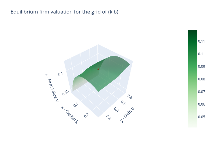
In the above 3D surface of prospective firm valuations, the perturbed choice \((k^*,b^{*}-e)\), represented by the red dot, is not at the top.
The firm could issue more debts and attain a higher firm valuation from the market.
Therefore, \((k^*,b^{*}-e)\) would not be an equilibrium.
Next, we check for \(b^{**} = b^* + e\).
#====================== Experiment 2 ======================#
Ve2,ke2,be2,pe2,qe2,c10e2,c11e2,c20e2,c21e2,𝜉1e2 = off_eq_check(mdl,
                                                                kss,
                                                                bss,
                                                                e=0.1)

# Firm Valuation
kgride2, bgride2, Vgride2, Qgride2, Pgride2 = mdl.eq_valuation(c10e2, c11e2, c20e2, c21e2,N=20)

print('Maximum valuation of the firm value in the (k,b) grid: {:.4f}'.format(Vgride2.max()))
print('Equilibrium firm value: {:.4f}'.format(Ve2))

fig = go.Figure(data=[go.Scatter3d(x=[ke2],
                                   y=[be2],
                                   z=[Ve2],
                                   mode='markers',
                                   marker=dict(size=3, color='red')),
                      go.Surface(x=kgride2,
                                 y=bgride2,
                                 z=Vgride2,
                                 colorscale='Greens',opacity=0.6)])

fig.update_layout(scene = dict(
                    xaxis_title='x - Capital k',
                    yaxis_title='y - Debt b',
                    zaxis_title='z - Firm Value V',
                    aspectratio = dict(x=1,y=1,z=1)),
                  width=700,
                  height=700,
                  margin=dict(l=50, r=50, b=65, t=90))
fig.update_layout(scene_camera=dict(eye=dict(x=1.5, y=-1.5, z=2)))
fig.update_layout(title='Equilibrium firm valuation for the grid of (k,b)')

# Export to PNG file
Image(fig.to_image(format="png", engine="kaleido"))
# fig.show() will provide interactive plot when running
# code locally
Maximum valuation of the firm value in the (k,b) grid: 0.1082
Equilibrium firm value: 0.0974
/tmp/ipykernel_6296/1131724249.py:35: DeprecationWarning:


Support for the 'engine' argument is deprecated and will be removed after September 2025.
Kaleido will be the only supported engine at that time.
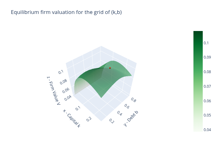
In contrast to \((k^*,b^* - e)\), the 3D surface for \((k^*,b^*+e)\) now indicates that a firm would want o decrease its debt issuance to attain a higher valuation.
That incentive to deviate means that \((k^*,b^*+e)\) is not an equilibrium capital structure for the firm.
Interestingly, if consumers were to anticipate that firms would over-issue debt, i.e. \(B > b^*\), then both types of consumer would want to hold corporate debt.
For example, \(\xi^1 > 0\):
print('Bond holdings of agent 1: {:.3f}'.format(𝜉1e2))
Bond holdings of agent 1: 0.039
Our two stability experiments suggest that the equilibrium capital structure \((k^*,b^*)\) is locally unique even though at the equilibrium an individual firm would be willing to deviate from the representative firms’ equilibrium debt choice.
These experiments thus refine our discussion of the qualified Modigliani-Miller theorem that prevails in this example economy.
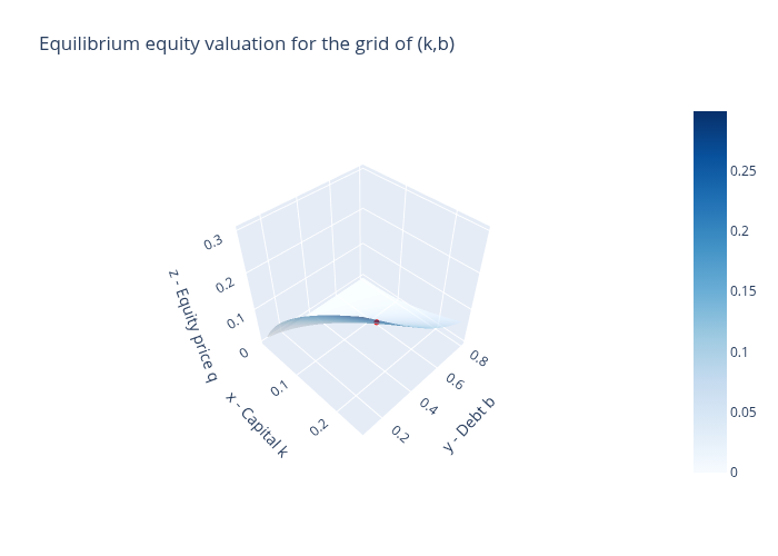
49.6.1.2. Equilibrium equity and bond price functions#
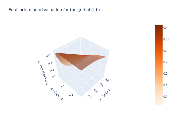
It is also interesting to look at the equilibrium price functions \(q(k,b)\) and \(p(k,b)\) faced by firms in our rational expectations equilibrium.
# Equity Valuation
fig = go.Figure(data=[go.Scatter3d(x=[kss],
                                   y=[bss],
                                   z=[qss],
                                   mode='markers',
                                   marker=dict(size=3, color='red')),
                      go.Surface(x=kgrid,
                                 y=bgrid,
                                 z=Qgrid,
                                 colorscale='Blues',opacity=0.6)])

fig.update_layout(scene = dict(
                    xaxis_title='x - Capital k',
                    yaxis_title='y - Debt b',
                    zaxis_title='z - Equity price q',
                    aspectratio = dict(x=1,y=1,z=1)),
                  width=700,
                  height=700,
                  margin=dict(l=50, r=50, b=65, t=90))
fig.update_layout(scene_camera=dict(eye=dict(x=1.5, y=-1.5, z=2)))
fig.update_layout(title='Equilibrium equity valuation for the grid of (k,b)')


# Export to PNG file
Image(fig.to_image(format="png", engine="kaleido"))
# fig.show() will provide interactive plot when running
# code locally
/tmp/ipykernel_6296/2737751049.py:25: DeprecationWarning:


Support for the 'engine' argument is deprecated and will be removed after September 2025.
Kaleido will be the only supported engine at that time.
# Bond Valuation
fig = go.Figure(data=[go.Scatter3d(x=[kss],
                                   y=[bss],
                                   z=[pss],
                                   mode='markers',
                                   marker=dict(size=3, color='red')),
                      go.Surface(x=kgrid,
                                 y=bgrid,
                                 z=Pgrid,
                                 colorscale='Oranges',opacity=0.6)])

fig.update_layout(scene = dict(
                    xaxis_title='x - Capital k',
                    yaxis_title='y - Debt b',
                    zaxis_title='z - Bond price q',
                    aspectratio = dict(x=1,y=1,z=1)),
                  width=700,
                  height=700,
                  margin=dict(l=50, r=50, b=65, t=90))
fig.update_layout(scene_camera=dict(eye=dict(x=1.5, y=-1.5, z=2)))
fig.update_layout(title='Equilibrium bond valuation for the grid of (k,b)')


# Export to PNG file
Image(fig.to_image(format="png", engine="kaleido"))
# fig.show() will provide interactive plot when running
# code locally
/tmp/ipykernel_6296/2980259825.py:25: DeprecationWarning:


Support for the 'engine' argument is deprecated and will be removed after September 2025.
Kaleido will be the only supported engine at that time.
49.6.3. Another example economy#
We illustrate how the fraction of initial endowments held by agent 2, \(w^2_0/(w^1_0+w^2_0)\) affects an equilibrium capital structure \((k,b) = (K, B)\) well as associated equilibrium allocations.
We are interested in how agents 1 and 2 value equity and bond.
The function valuations_by_agent is used in calculating these
valuations.
# Lists for storage
wlist = []
klist = []
blist = []
qlist = []
plist = []
Vlist = []
tlist = []
q1list = []
q2list = []
p1list = []
p2list = []

# For loop: optimization for each endowment combination
for i in range(10):
    print(i)

    # Save fraction
    w10 = 0.9 - 0.05*i
    w20 = 1.1 + 0.05*i
    wlist.append(w20/(w10+w20))

    # Create the instance
    mdl = BCG_incomplete_markets(w10 = w10, w20 = w20, ktop = 0.5, btop = 2.5)

    # Solve for equilibrium
    kss,bss,Vss,qss,pss,c10ss,c11ss,c20ss,c21ss,𝜃1ss = mdl.solve_eq(print_crit=False)

    # Store the equilibrium results
    klist.append(kss)
    blist.append(bss)
    qlist.append(qss)
    plist.append(pss)
    Vlist.append(Vss)
    tlist.append(𝜃1ss)

    # Evaluations of equity and bond by each agent
    Q1,Q2,P1,P2 = mdl.valuations_by_agent(c10ss, c11ss, c20ss, c21ss, kss, bss)

    # Save the valuations
    q1list.append(Q1)
    q2list.append(Q2)
    p1list.append(P1)
    p2list.append(P2)
# Plot
fig, ax = plt.subplots(3,2,figsize=(12,12))
ax[0,0].plot(wlist,klist)
ax[0,0].set_title('capital')
ax[0,1].plot(wlist,blist)
ax[0,1].set_title('debt')
ax[1,0].plot(wlist,qlist)
ax[1,0].set_title('equity price')
ax[1,1].plot(wlist,plist)
ax[1,1].set_title('bond price')
ax[2,0].plot(wlist,Vlist)
ax[2,0].set_title('firm value')
ax[2,0].set_xlabel('fraction of initial endowment held by agent 2',fontsize=13)

# Create a list of Default thresholds
A = mdl.A
𝛼 = mdl.𝛼
epslist = []
for i in range(len(wlist)):
    bb = blist[i]
    kk = klist[i]
    eps = np.log(bb/(A*kk**𝛼))
    epslist.append(eps)

# Plot (cont.)
ax[2,1].plot(wlist,epslist)
ax[2,1].set_title(r'default threshold $\epsilon^*$')
ax[2,1].set_xlabel('fraction of initial endowment held by agent 2',fontsize=13)
plt.show()
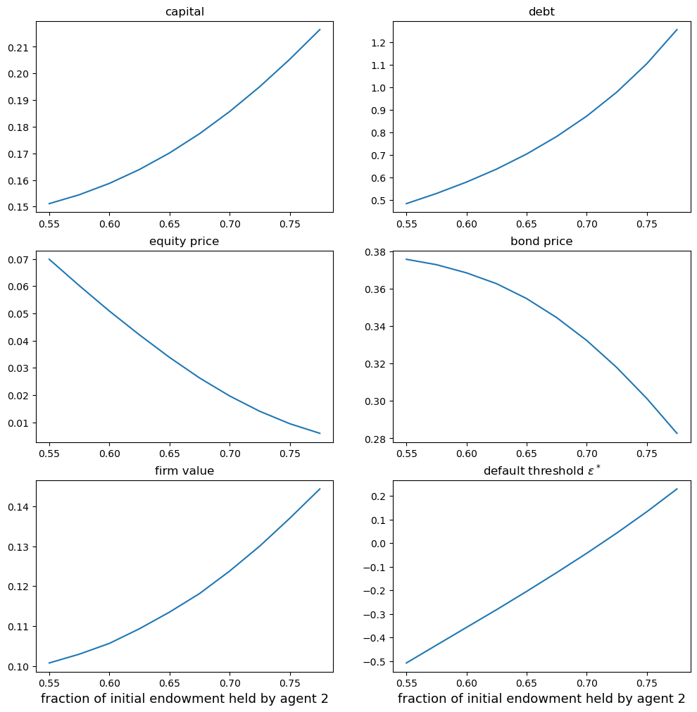
49.7. A picture worth a thousand words#
Please stare at the above panels.
They describe how equilibrium prices and quantities respond to alterations in the structure of society’s hedging desires across economies with different allocations of the initial endowment to our two types of agents.
Now let’s see how the two types of agents value bonds and equities, keeping in mind that the type that values the asset highest determines the equilibrium price (and thus the pertinent set of Big \(C\)’s).
# Comparing the prices
fig, ax = plt.subplots(1,3,figsize=(16,6))

ax[0].plot(wlist,q1list,label='agent 1',color='green')
ax[0].plot(wlist,q2list,label='agent 2',color='blue')
ax[0].plot(wlist,qlist,label='equity price',color='red',linestyle='--')
ax[0].legend()
ax[0].set_title('equity valuations')
ax[0].set_xlabel('fraction of initial endowment held by agent 2',fontsize=11)

ax[1].plot(wlist,p1list,label='agent 1',color='green')
ax[1].plot(wlist,p2list,label='agent 2',color='blue')
ax[1].plot(wlist,plist,label='bond price',color='red',linestyle='--')
ax[1].legend()
ax[1].set_title('bond valuations')
ax[1].set_xlabel('fraction of initial endowment held by agent 2',fontsize=11)

ax[2].plot(wlist,tlist,color='blue')
ax[2].set_title('equity holdings by agent 1')
ax[2].set_xlabel('fraction of initial endowment held by agent 2',fontsize=11)

plt.show()
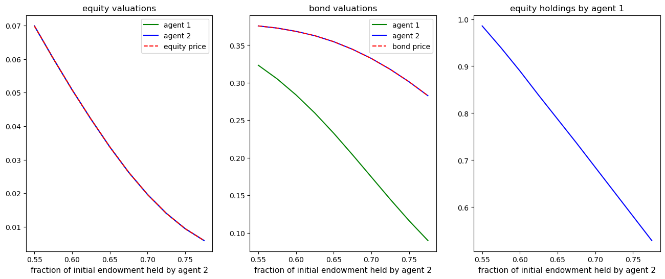
It is rewarding to stare at the above plots too.
In equilibrium, equity valuations are the same across the two types of agents but bond valuations are not.
Agents of type 2 value bonds more highly (they want more hedging).
Taken together with our earlier plot of equity holdings, these graphs confirm our earlier conjecture that while both type of agents hold equities, only agents of type 2 holds bonds.
49.6.2. Comments on equilibrium pricing functions#
The equilibrium pricing functions displayed above merit study and reflection.
They reveal the countervailing effects on a firm’s valuations of bonds and equities that lie beneath the Modigliani-Miller ridge apparent in our earlier graph of an individual firm \(\zeta\)’s value as a function of \(k(\zeta), b(\zeta)\).