11. How to Pay for a War: Part 3 #

Contents

How to Pay for a War: Part 3

In addition to what’s in Anaconda, this lecture deploys the quantecon library:

!pip install --upgrade quantecon

11.1. Another Application of Markov Jump Linear Quadratic Dynamic Programming #

This is another sequel to an earlier lecture.

We again use a method introduced in lecture Markov Jump LQ dynamic programming to implement some ideas Barro (1999 [Bar99], 2003 [BM03]) that extend his classic 1979 [Bar79] model of tax smoothing.

Barro’s 1979 [Bar79] model is about a government that borrows and lends in order to help it minimize an intertemporal measure of distortions caused by taxes.

Technically, Barro’s 1979 [Bar79] model looks a lot like a consumption-smoothing model.

Our generalizations of his 1979 model will also look like souped-up consumption-smoothing models.

In this lecture, we describe a tax-smoothing problem of a government that faces roll-over risk.

Let’s start with some standard imports:

import quantecon as qe
import numpy as np
import matplotlib.pyplot as plt
%matplotlib inline

11.2. Roll-Over Risk #

Let \(T_t\) denote tax collections, \(\beta\) a discount factor, \(b_{t,t+1}\) time \(t+1\) goods that the government promises to pay at \(t\), \(G_t\) government purchases, \(p^t_{t+1}\) the number of time \(t\) goods received per time \(t+1\) goods promised.

The stochastic process of government expenditures is exogenous.

The government’s problem is to choose a plan for borrowing and tax collections \(\{b_{t+1}, T_t\}_{t=0}^\infty\) to minimize

\[ E_0 \sum_{t=0}^\infty \beta^t T_t^2 \]

subject to the constraints

\[ T_t + p^t_{t+1} b_{t,t+1} = G_t + b_{t-1,t} \]

\[ G_t = U_{g,t} z_t \]

\[ z_{t+1} = A_{22,t} z_t + C_{2,t} w_{t+1} \]

where \(w_{t+1} \sim {\cal N}(0,I)\). The variables \(T_t, b_{t, t+1}\) are control variables chosen at \(t\), while \(b_{t-1,t}\) is an endogenous state variable inherited from the past at time \(t\) and \(p^t_{t+1}\) is an exogenous state variable at time \(t\).

This is the same set-up as used in this lecture.

We will consider a situation in which the government faces “roll-over risk”.

Specifically, we shut down the government’s ability to borrow in one of the Markov states.

11.3. A Dead End #

A first thought for how to implement this might be to allow \(p^t_{t+1}\) to vary over time with:

\[ p^t_{t+1} = \beta \]

in Markov state 1 and

\[ p^t_{t+1} = 0 \]

in Markov state 2.

Consequently, in the second Markov state, the government is unable to borrow, and the budget constraint becomes \(T_t = G_t + b_{t-1,t}\).

However, if this is the only adjustment we make in our linear-quadratic model, the government will not set \(b_{t,t+1} = 0\), which is the outcome we want to express roll-over risk in period \(t\).

Instead, the government would have an incentive to set \(b_{t,t+1}\) to a large negative number in state 2 – it would accumulate large amounts of assets to bring into period \(t+1\) because that is cheap (Our Riccati equations will discover this for us!).

Thus, we must represent “roll-over risk” some other way.

11.4. Better Representation of Roll-Over Risk #

To force the government to set \(b_{t,t+1} = 0\), we can instead extend the model to have four Markov states:

Good today, good yesterday
Good today, bad yesterday
Bad today, good yesterday
Bad today, bad yesterday

where good is a state in which effectively the government can issue debt and bad is a state in which effectively the government can’t issue debt.

We’ll explain what effectively means shortly.

We now set

\[ p^t_{t+1} = \beta \]

in all states.

In addition – and this is important because it defines what we mean by effectively – we put a large penalty on the \(b_{t-1,t}\) element of the state vector in states 2 and 4.

This will prevent the government from wishing to issue any debt in states 3 or 4 because it would experience a large penalty from doing so in the next period.

The transition matrix for this formulation is:

\[\begin{split} \Pi = \begin{bmatrix} 0.95 & 0 & 0.05 & 0 \\ 0.95 & 0 & 0.05 & 0 \\ 0 & 0.9 & 0 & 0.1 \\ 0 & 0.9 & 0 & 0.1 \\ \end{bmatrix} \end{split}\]

This transition matrix ensures that the Markov state cannot move, for example, from state 3 to state 1.

Because state 3 is “bad today”, the next period cannot have “good yesterday”.

# Model parameters
β, Gbar, ρ, σ = 0.95, 5, 0.8, 1

# Basic model matrices
A22 = np.array([[1, 0], [Gbar, ρ], ])
C2 = np.array([[0], [σ]])
Ug = np.array([[0, 1]])

# LQ framework matrices
A_t = np.zeros((1, 3))
A_b = np.hstack((np.zeros((2, 1)), A22))
A = np.vstack((A_t, A_b))

B = np.zeros((3, 1))
B[0, 0] = 1

C = np.vstack((np.zeros((1, 1)), C2))

Sg = np.hstack((np.zeros((1, 1)), Ug))
S1 = np.zeros((1, 3))
S1[0, 0] = 1
S = S1 + Sg

R = S.T @ S

# Large penalty on debt in R2 to prevent borrowing in a bad state
R1 = np.copy(R)
R2 = np.copy(R)
R1[0, 0] = R[0, 0] + 1e-9
R2[0, 0] = R[0, 0] + 1e12

M = np.array([[-β]])
Q = M.T @ M
W = M.T @ S

Π = np.array([[0.95,   0, 0.05,   0],
              [0.95,   0, 0.05,   0],
              [0,    0.9,    0, 0.1],
              [0,    0.9,    0, 0.1]])

# Construct lists of matrices that correspond to each state
As = [A, A, A, A]
Bs = [B, B, B, B]
Cs = [C, C, C, C]
Rs = [R1, R2, R1, R2]
Qs = [Q, Q, Q, Q]
Ws = [W, W, W, W]

lqm = qe.LQMarkov(Π, Qs, Rs, As, Bs, Cs=Cs, Ns=Ws, beta=β)
lqm.stationary_values();

This model is simulated below, using the same process for \(G_t\) as in this lecture.

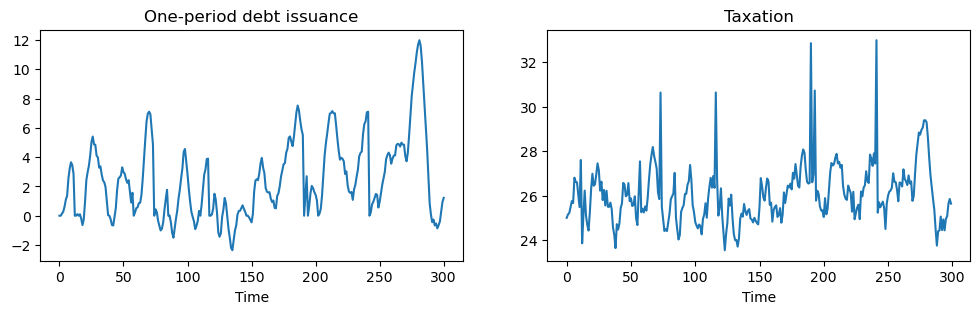
When \(p^t_{t+1} = \beta\) government debt fluctuates around zero.

The spikes in the series for taxation show periods when the government is unable to access financial markets: positive spikes occur when debt is positive, and the government must raise taxes in the current period.

Negative spikes occur when the government has positive asset holdings.

An inability to use financial markets in the next period means that the government uses those assets to lower taxation today.

x0 = np.array([[0, 1, 25]])
T = 300
x, u, w, state = lqm.compute_sequence(x0, ts_length=T)

# Calculate taxation each period from the budget constraint and the Markov state
tax = np.zeros([T, 1])
for i in range(T):
    tax[i, :] = S @ x[:, i] + M @ u[:, i]

# Plot of debt issuance and taxation
fig, (ax1, ax2) = plt.subplots(1, 2, figsize=(12, 3))
ax1.plot(x[0, :])
ax1.set_title('One-period debt issuance')
ax1.set_xlabel('Time')
ax2.plot(tax)
ax2.set_title('Taxation')
ax2.set_xlabel('Time')
plt.show()

_images/53a4a9bb0bf8dd74268ac4502523aaf80e34eb36e7f751f1dc7016b72ba9f13e.png

We can adjust the model so that, rather than having debt fluctuate around zero, the government is a debtor in every period we allow it to borrow.

To accomplish this, we simply raise \(p^t_{t+1}\) to \(\beta + 0.02 = 0.97\).

M = np.array([[-β - 0.02]])

Q = M.T @ M
W = M.T @ S

# Construct lists of matrices
As = [A, A, A, A]
Bs = [B, B, B, B]
Cs = [C, C, C, C]
Rs = [R1, R2, R1, R2]
Qs = [Q, Q, Q, Q]
Ws = [W, W, W, W]

lqm2 = qe.LQMarkov(Π, Qs, Rs, As, Bs, Cs=Cs, Ns=Ws, beta=β)
x, u, w, state = lqm2.compute_sequence(x0, ts_length=T)

# Calculate taxation each period from the budget constraint and the
# Markov state
tax = np.zeros([T, 1])
for i in range(T):
    tax[i, :] = S @ x[:, i] + M @ u[:, i]

# Plot of debt issuance and taxation
fig, (ax1, ax2) =  plt.subplots(1, 2, figsize=(12, 3))
ax1.plot(x[0, :])
ax1.set_title('One-period debt issuance')
ax1.set_xlabel('Time')
ax2.plot(tax)
ax2.set_title('Taxation')
ax2.set_xlabel('Time')
plt.show()

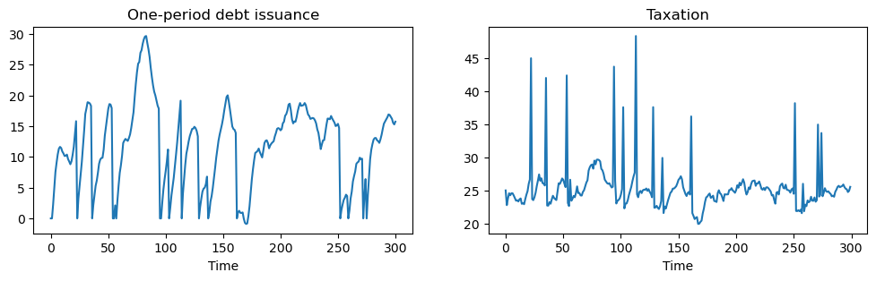
_images/5776de8bcfb8477ff8272779af2fcc9243ae5761141fc0169223d0737937a1eb.png

With a lower interest rate, the government has an incentive to increase debt over time.

However, with “roll-over risk”, debt is recurrently reset to zero and taxes spike up.

Consequently, the government is wary of letting debt get too high, due to the high costs of a “sudden stop”.

11. How to Pay for a War: Part 3#

11.1. Another Application of Markov Jump Linear Quadratic Dynamic Programming#

11.2. Roll-Over Risk#

11.3. A Dead End#

11.4. Better Representation of Roll-Over Risk#

11. How to Pay for a War: Part 3 #

11.1. Another Application of Markov Jump Linear Quadratic Dynamic Programming #

11.2. Roll-Over Risk #

11.3. A Dead End #

11.4. Better Representation of Roll-Over Risk #