3. Reverse Engineering a la Muth #

Contents

Reverse Engineering a la Muth

In addition to what’s in Anaconda, this lecture uses the quantecon library.

!pip install --upgrade quantecon

We’ll also need the following imports:

import matplotlib.pyplot as plt
%matplotlib inline
import numpy as np

from quantecon import Kalman
from quantecon import LinearStateSpace
np.set_printoptions(linewidth=120, precision=4, suppress=True)

This lecture uses the Kalman filter to reformulate John F. Muth’s first paper [Mut60] about rational expectations.

Muth used classical prediction methods to reverse engineer a stochastic process that renders optimal Milton Friedman’s [Fri56] “adaptive expectations” scheme.

3.1. Friedman (1956) and Muth (1960)#

Milton Friedman [Fri56] (1956) posited that consumer’s forecast their future disposable income with the adaptive expectations scheme

(3.1)#\[y_{t+i,t}^* = K \sum_{j=0}^\infty (1 - K)^j y_{t-j}\]

where \(K \in (0,1)\) and \(y_{t+i,t}^*\) is a forecast of future \(y\) over horizon \(i\).

Milton Friedman justified the exponential smoothing forecasting scheme (3.1) informally, noting that it seemed a plausible way to use past income to forecast future income.

In his first paper about rational expectations, John F. Muth [Mut60] reverse-engineered a univariate stochastic process \(\{y_t\}_{t=- \infty}^\infty\) for which Milton Friedman’s adaptive expectations scheme gives linear least forecasts of \(y_{t+j}\) for any horizon \(i\).

Muth sought a setting and a sense in which Friedman’s forecasting scheme is optimal.

That is, Muth asked for what optimal forecasting question is Milton Friedman’s adaptive expectation scheme the answer.

Muth (1960) used classical prediction methods based on lag-operators and \(z\)-transforms to find the answer to his question.

Please see lectures Classical Control with Linear Algebra and Classical Filtering and Prediction with Linear Algebra for an introduction to the classical tools that Muth used.

Rather than using those classical tools, in this lecture we apply the Kalman filter to express the heart of Muth’s analysis concisely.

The lecture First Look at Kalman Filter describes the Kalman filter.

We’ll use limiting versions of the Kalman filter corresponding to what are called stationary values in that lecture.

3.2. A Process for Which Adaptive Expectations are Optimal #

Suppose that an observable \(y_t\) is the sum of an unobserved random walk \(x_t\) and an IID shock \(\epsilon_{2,t}\):

(3.2)#\[\begin{aligned} x_{t+1} & = x_t + \sigma_x \epsilon_{1,t+1} \cr y_t & = x_t + \sigma_y \epsilon_{2,t} \end{aligned}\]

where

\[ \begin{bmatrix} \epsilon_{1,t+1} \cr \epsilon_{2,t} \end{bmatrix} \sim {\mathcal N} (0, I) \]

is an IID process.

Note

A property of the state-space representation (3.2) is that in general neither \(\epsilon_{1,t}\) nor \(\epsilon_{2,t}\) is in the space spanned by square-summable linear combinations of \(y_t, y_{t-1}, \ldots\).

In general \(\begin{bmatrix} \epsilon_{1,t} \cr \epsilon_{2t} \end{bmatrix}\) has more information about future \(y_{t+j}\)’s than is contained in \(y_t, y_{t-1}, \ldots\).

We can use the asymptotic or stationary values of the Kalman gain and the one-step-ahead conditional state covariance matrix to compute a time-invariant innovations representation

(3.3)#\[\begin{aligned} \hat x_{t+1} & = \hat x_t + K a_t \cr y_t & = \hat x_t + a_t \end{aligned}\]

where \(\hat x_t = E [x_t | y_{t-1}, y_{t-2}, \ldots ]\) and \(a_t = y_t - E[y_t |y_{t-1}, y_{t-2}, \ldots ]\).

Note

A key property about an innovations representation is that \(a_t\) is in the space spanned by square summable linear combinations of \(y_t, y_{t-1}, \ldots\).

For more ramifications of this property, see the lectures Shock Non-Invertibility and Recursive Models of Dynamic Linear Economies.

Later we’ll stack these state-space systems (3.2) and (3.3) to display some classic findings of Muth.

But first, let’s create an instance of the state-space system (3.2) then apply the quantecon Kalman class, then uses it to construct the associated “innovations representation”

# Make some parameter choices
# sigx/sigy are state noise std err and measurement noise std err
μ_0, σ_x, σ_y = 10, 1, 5

# Create a LinearStateSpace object
A, C, G, H = 1, σ_x, 1, σ_y
ss = LinearStateSpace(A, C, G, H, mu_0=μ_0)

# Set prior and initialize the Kalman type
x_hat_0, Σ_0 = 10, 1
kmuth = Kalman(ss, x_hat_0, Σ_0)

# Computes stationary values which we need for the innovation
# representation
S1, K1 = kmuth.stationary_values()

# Extract scalars from nested arrays
S1, K1 = S1.item(), K1.item()

# Form innovation representation state-space
Ak, Ck, Gk, Hk = A, K1, G, 1

ssk = LinearStateSpace(Ak, Ck, Gk, Hk, mu_0=x_hat_0)

3.3. Some Useful State-Space Math #

Now we want to map the time-invariant innovations representation (3.3) and the original state-space system (3.2) into a convenient form for deducing the impulse responses from the original shocks to the \(x_t\) and \(\hat x_t\).

Putting both of these representations into a single state-space system is yet another application of the insight that “finding the state is an art”.

We’ll define a state vector and appropriate state-space matrices that allow us to represent both systems in one fell swoop.

Note that

\[ a_t = x_t + \sigma_y \epsilon_{2,t} - \hat x_t \]

so that

\[ \begin{aligned} \hat x_{t+1} & = \hat x_t + K (x_t + \sigma_y \epsilon_{2,t} - \hat x_t) \cr & = (1-K) \hat x_t + K x_t + K \sigma_y \epsilon_{2,t} \end{aligned} \]

The stacked system

\[ \begin{bmatrix} x_{t+1} \cr \hat x_{t+1} \cr \epsilon_{2,t+1} \end{bmatrix} = \begin{bmatrix} 1 & 0 & 0 \cr K & (1-K) & K \sigma_y \cr 0 & 0 & 0 \end{bmatrix} \begin{bmatrix} x_{t} \cr \hat x_t \cr \epsilon_{2,t} \end{bmatrix}+ \begin{bmatrix} \sigma_x & 0 \cr 0 & 0 \cr 0 & 1 \end{bmatrix} \begin{bmatrix} \epsilon_{1,t+1} \cr \epsilon_{2,t+1} \end{bmatrix} \]

\[ \begin{bmatrix} y_t \cr a_t \end{bmatrix} = \begin{bmatrix} 1 & 0 & \sigma_y \cr 1 & -1 & \sigma_y \end{bmatrix} \begin{bmatrix} x_{t} \cr \hat x_t \cr \epsilon_{2,t} \end{bmatrix} \]

is a state-space system that tells us how the shocks \(\begin{bmatrix} \epsilon_{1,t+1} \cr \epsilon_{2,t+1} \end{bmatrix}\) affect states \(\hat x_{t+1}, x_t\), the observable \(y_t\), and the innovation \(a_t\).

With this tool at our disposal, let’s form the composite system and simulate it

# Create grand state-space for y_t, a_t as observed vars -- Use
# stacking trick above
Af = np.array([[ 1,      0,        0],
               [K1, 1 - K1, K1 * σ_y],
               [ 0,      0,        0]])
Cf = np.array([[σ_x,        0],
               [  0, K1 * σ_y],
               [  0,        1]])
Gf = np.array([[1,  0, σ_y],
               [1, -1, σ_y]])

μ_true, μ_prior = 10, 10
μ_f = np.array([μ_true, μ_prior, 0]).reshape(3, 1)

# Create the state-space
ssf = LinearStateSpace(Af, Cf, Gf, mu_0=μ_f)

# Draw observations of y from the state-space model
N = 50
xf, yf = ssf.simulate(N)

print(f"Kalman gain = {K1}")
print(f"Conditional variance = {S1}")

Kalman gain = 0.1809975124224177
Conditional variance = 5.524937810560442

Now that we have simulated our joint system, we have \(x_t\), \(\hat{x_t}\), and \(y_t\).

We can now investigate how these variables are related by plotting some key objects.

3.4. Estimates of Unobservables #

First, let’s plot the hidden state \(x_t\) and the filtered version \(\hat x_t\) that is linear-least squares projection of \(x_t\) on the history \(y_{t-1}, y_{t-2}, \ldots\)

fig, ax = plt.subplots()
ax.plot(xf[0, :], label="$x_t$")
ax.plot(xf[1, :], label="Filtered $x_t$")
ax.legend()
ax.set_xlabel("Time")
ax.set_title(r"$x$ vs $\hat{x}$")
plt.show()

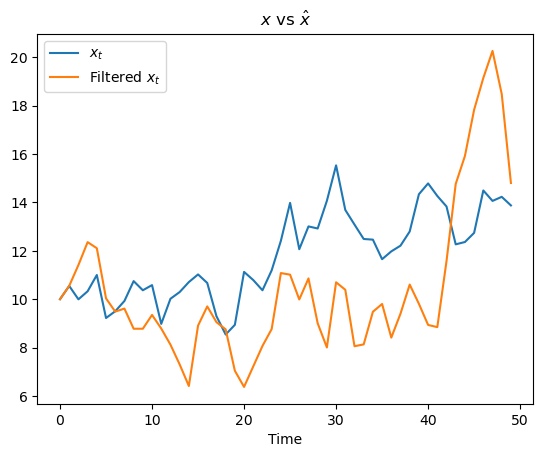
_images/e1c6d135020a02d252444d55be05477f470dc60d953b2153763aab3ce806a5e0.png

Note how \(x_t\) and \(\hat{x_t}\) differ.

For Friedman, \(\hat x_t\) and not \(x_t\) is the consumer’s idea about her/his permanent income.

3.5. Relationship of Unobservables to Observables #

Now let’s plot \(x_t\) and \(y_t\).

Recall that \(y_t\) is just \(x_t\) plus white noise

fig, ax = plt.subplots()
ax.plot(yf[0, :], label="y")
ax.plot(xf[0, :], label="x")
ax.legend()
ax.set_title(r"$x$ and $y$")
ax.set_xlabel("Time")
plt.show()

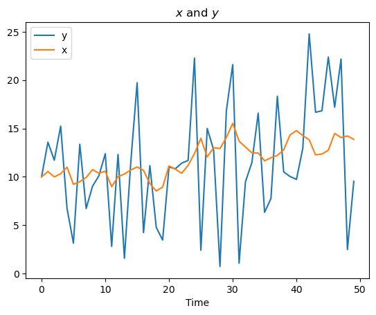
_images/a1ffa627baaa0da4933dc4b48e5023f063dd61221073d3cbb9ac78b39ec10a4f.png

We see above that \(y\) seems to look like white noise around the values of \(x\).

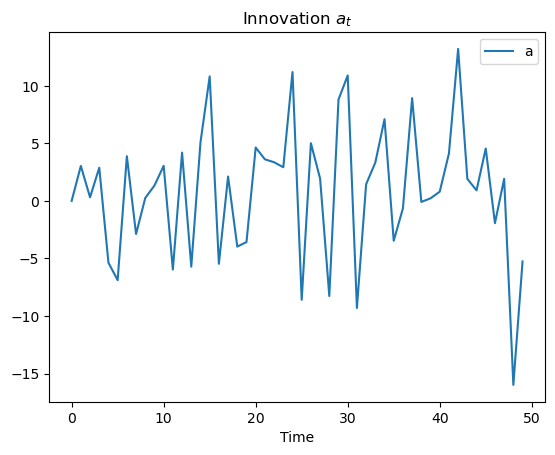
3.5.1. Innovations#

Recall that we wrote down the innovation representation that depended on \(a_t\). We now plot the innovations \(\{a_t\}\):

fig, ax = plt.subplots()
ax.plot(yf[1, :], label="a")
ax.legend()
ax.set_title(r"Innovation $a_t$")
ax.set_xlabel("Time")
plt.show()

_images/ef92ceb91d6818b5a0f31755dae9392a0f45802c63dacd90f312cbdbf13ecfb0.png

3.6. MA and AR Representations #

Now we shall extract from the Kalman instance kmuth coefficients of

a fundamental moving average representation that represents \(y_t\) as a one-sided moving sum of current and past \(a_t\)s that are square summable linear combinations of \(y_t, y_{t-1}, \ldots\).
a univariate autoregression representation that depicts the coefficients in a linear least square projection of \(y_t\) on the semi-infinite history \(y_{t-1}, y_{t-2}, \ldots\).

Then we’ll plot each of them

# Kalman Methods for MA and VAR
coefs_ma = kmuth.stationary_coefficients(5, "ma")
coefs_var = kmuth.stationary_coefficients(5, "var")

# Coefficients come in a list of arrays, but we
# want to plot them and so need to stack into an array
coefs_ma_array = np.vstack(coefs_ma)
coefs_var_array = np.vstack(coefs_var)

fig, ax = plt.subplots(2)
ax[0].plot(coefs_ma_array, label="MA")
ax[0].legend()
ax[1].plot(coefs_var_array, label="VAR")
ax[1].legend()

plt.show()

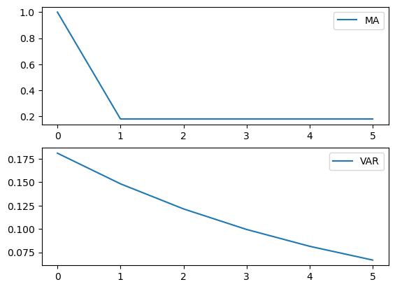
_images/b3879b9ad60f75b2b4d6b7db6ef97c4a56457cfde5e27f7e3e4915afb9acdd84.png

The moving average coefficients in the top panel show tell-tale signs of \(y_t\) being a process whose first difference is a first-order autoregression.

The autoregressive coefficients decline geometrically with decay rate \((1-K)\).

These are exactly the target outcomes that Muth (1960) aimed to reverse engineer

print(f'decay parameter 1 - K1 = {1 - K1}')

decay parameter 1 - K1 = 0.8190024875775823

3. Reverse Engineering a la Muth#

3.1. Friedman (1956) and Muth (1960)#

3.2. A Process for Which Adaptive Expectations are Optimal#

3.3. Some Useful State-Space Math#

3.4. Estimates of Unobservables#

3.5. Relationship of Unobservables to Observables#

3.5.1. Innovations#

3.6. MA and AR Representations#

3. Reverse Engineering a la Muth #

3.2. A Process for Which Adaptive Expectations are Optimal #

3.3. Some Useful State-Space Math #

3.4. Estimates of Unobservables #

3.5. Relationship of Unobservables to Observables #

3.6. MA and AR Representations #