38. Knowing the Forecasts of Others#
In addition to what’s in Anaconda, this lecture will need the following libraries:
!pip install --upgrade quantecon
!conda install -y -c plotly plotly plotly-orca
38.1. Introduction#
Robert E. Lucas, Jr. [Robert E. Lucas, 1975], Kenneth Kasa [Kasa, 2000], and Robert Townsend [Townsend, 1983] showed that putting decision makers into environments in which they want to infer persistent hidden state variables from equilibrium prices and quantities can elongate and amplify impulse responses to aggregate shocks.
This provides a promising way to think about amplification mechanisms in business cycle models.
Townsend [Townsend, 1983] noted that living in such environments makes decision makers want to forecast forecasts of others.
This theme has been pursued for situations in which decision makers’ imperfect information forces them to pursue an infinite recursion that involves forming beliefs about the beliefs of others (e.g., [Allen et al., 2002]).
Lucas [Robert E. Lucas, 1975] side stepped having decision makers forecast the forecasts of other decision makers by assuming that they simply pool their information before forecasting.
A pooling equilibrium like Lucas’s plays a prominent role in this lecture.
Because he didn’t assume such pooling, [Townsend, 1983] confronted the forecasting the forecasts of others problem.
To formulate the problem recursively required that Townsend define a decision maker’s state vector.
Townsend concluded that his original model required an intractable infinite dimensional state space.
Therefore, he constructed a more manageable approximating model in which a hidden Markov component of a demand shock is revealed to all firms after a fixed, finite number of periods.
In this lecture, we illustrate again the theme that finding the state is an art by showing how to formulate Townsend’s original model in terms of a low-dimensional state space.
We show that Townsend’s model shares equilibrium prices and quantities with those that prevail in a pooling equilibrium.
That finding emerged from a line of research about Townsend’s model that built on [Pearlman et al., 1986] and that culminated in [Pearlman and Sargent, 2005] .
Rather than directly deploying the [Pearlman et al., 1986] machinery here, we shall instead implement a sneaky guess-and-verify tactic.
We first compute a pooling equilibrium and represent it as an instance of a linear state-space system provided by the Python class
quantecon.LinearStateSpace.Leaving the state-transition equation for the pooling equilibrium unaltered, we alter the observation vector for a firm to match what it is in Townsend’s original model. So rather than directly observing the signal received by firms in the other industry, a firm sees the equilibrium price of the good produced by the other industry.
We compute a population linear least squares regression of the noisy signal at time \(t\) that firms in the other industry would receive in a pooling equilibrium on time \(t\) information that a firm receives in Townsend’s original model.
The \(R^2\) in this regression equals \(1\).
That verifies that a firm’s information set in Townsend’s original model equals its information set in a pooling equilibrium.
Therefore, equilibrium prices and quantities in Townsend’s original model equal those in a pooling equilibrium.
38.1.1. A sequence of models#
We proceed by describing a sequence of models of two industries that are linked in a single way:
shocks to the demand curves for their products have a common component.
The models are simplified versions of Townsend’s [Townsend, 1983].
Townsend’s is a model of a rational expectations equilibrium in which firms want to forecast forecasts of others.
In Townsend’s model, firms condition their forecasts on observed endogenous variables whose equilibrium laws of motion are determined by their own forecasting functions.
We shall assemble model components progressively in ways that can help us to appreciate the structure of the pooling equilibrium that ultimately interests us.
While keeping all other aspects of the model the same, we shall study consequences of alternative assumptions about what decision makers observe.
Technically, this lecture deploys concepts and tools that appear in First Look at Kalman Filter and Rational Expectations Equilibrium.
38.2. The setting#
We cast all variables in terms of deviations from means.
Therefore, we omit constants from inverse demand curves and other functions.
Firms in industry \(i=1,2\) use a single factor of production, capital \(k_t^i\), to produce output of a single good, \(y_t^i\).
Firms bear quadratic costs of adjusting their capital stocks.
A representative firm in industry \(i\) has production function \(y_t^i = f k_t^i\), \(f >0\).
The firm acts as a price taker with respect to output price \(P_t^i\), and maximizes
Demand in industry \(i\) is described by the inverse demand curve
where \(P_t^i\) is the price of good \(i\) at \(t\), \(Y_t^i = f K_t^i\) is output in market \(i\), \(\theta_t\) is a persistent component of a demand shock that is common across the two industries, and \(\epsilon_t^i\) is an industry specific component of the demand shock that is i.i.d. and whose time \(t\) marginal distribution is \({\mathcal N}(0, \sigma_{\epsilon}^2)\).
We assume that \(\theta_t\) is governed by
where \(\{v_{t}\}\) is an i.i.d. sequence of Gaussian shocks, each with mean zero and variance \(\sigma_v^2\).
To simplify notation, we’ll study a special case by setting \(h=f=1\).
Costs of adjusting their capital stocks impart to firms an incentive to forecast the price of the good that they sell.
Throughout, we use the rational expectations equilibrium concept presented in this lecture Rational Expectations Equilibrium.
We let capital letters denote market wide objects and lower case letters denote objects chosen by a representative firm.
In each industry, a competitive equilibrium prevails.
To rationalize the big \(K\), little \(k\) connection, we can think of there being a continuum of firms in industry \(i\), with each firm being indexed by \(\omega \in [0,1]\) and \(K^i = \int_0^1 k^i(\omega) d \omega\).
In equilibrium, \(k_t^i = K_t^i\), but we must distinguish between \(k_t^i\) and \(K_t^i\) when we pose the firm’s optimization problem.
38.3. Tactics#
We shall compute equilibrium laws of motion for capital in industry \(i\) under a sequence of assumptions about what a representative firm observes.
Successive members of this sequence make a representative firm’s information more and more obscure.
We begin with the most information, then gradually withdraw information in a way that approaches and eventually reaches the Townsend-like information structure that we are ultimately interested in.
Thus, we shall compute equilibria under the following alternative information structures:
Perfect foresight: future values of \(\theta_t, \epsilon_{t}^i\) are observed in industry \(i\).
Observed history of stochastic \(\theta_t\): \(\{\theta_t, \epsilon_{t}^i\}\) are realizations from a stochastic process; current and past values of each are observed at time \(t\) but future values are not.
One noise-ridden observation on \(\theta_t\): values of \(\{\theta_t, \epsilon_{t}^i\}\) separately are never observed. However, at time \(t\), a history \(w^t\) of scalar noise-ridden observations on \(\theta_t\) is observed at time \(t\).
Two noise-ridden observations on \(\theta_t\): values of \(\{\theta_t, \epsilon_{t}^i\}\) separately are never observed. However, at time \(t\), a history \(w^t\) of two noise-ridden observations on \(\theta_t\) is observed at time \(t\).
Successive computations build one on previous ones.
We proceed by first finding an equilibrium under perfect foresight.
To compute an equilibrium with current and past but not future values of \(\theta_t\) observed, we use a certainty equivalence principle to justify modifying the perfect foresight equilibrium by replacing future values of \(\theta_s, \epsilon_{s}^i, s \geq t\) with mathematical expectations conditioned on \(\theta_t\).
This provides the equilibrium when \(\theta_t\) is observed at \(t\) but future \(\theta_{t+j}\) and \(\epsilon_{t+j}^i\) are not observed.
To find an equilibrium when a history \(w^t\) observations of a single noise-ridden \(\theta_t\) is observed, we again apply a certainty equivalence principle and replace future values of the random variables \(\theta_s, \epsilon_{s}^i, s \geq t\) with their mathematical expectations conditioned on \(w^t\).
To find an equilibrium when a history \(w^t\) of two noisy signals on \(\theta_t\) is observed, we replace future values of the random variables \(\theta_s, \epsilon_{s}^i, s \geq t\) with their mathematical expectations conditioned on history \(w^t\).
We call the equilibrium with two noise-ridden observations on \(\theta_t\) a pooling equilibrium.
It corresponds to an arrangement in which at the beginning of each period firms in industries \(1\) and \(2\) somehow get together and share information about current values of their noisy signals on \(\theta\).
We want ultimately to compare outcomes in a pooling equilibrium with an equilibrium under the following alternative information structure for a firm in industry \(i\) that originally interested Townsend [Townsend, 1983]:
Firm \(i\)’s noise-ridden signal on \(\theta_t\) and the price in industry \(-i\), a firm in industry \(i\) observes a history \(w^t\) of one noise-ridden signal on \(\theta_t\) and a history of industry \(-i\)’s price is observed. (Here \(-i\) means ``not \(i\)’’.)
With this information structure, a representative firm \(i\) sees the price as well as the aggregate endogenous state variable \(Y_t^i\) in its own industry.
That allows it to infer the total demand shock \(\theta_t + \epsilon_{t}^i\).
However, at time \(t\), the firm sees only \(P_t^{-i}\) and does not see \(Y_t^{-i}\), so that a firm in industry \(i\) does not directly observe \(\theta_t + \epsilon_t^{-i}\).
Nevertheless, it will turn out that equilibrium prices and quantities in this equilibrium equal their counterparts in a pooling equilibrium because firms in industry \(i\) are able to infer the noisy signal about the demand shock received by firms in industry \(-i\).
We shall verify this assertion by using a guess and verify tactic that involves running a least squares regression and inspecting its \(R^2\). [1]
38.4. Equilibrium conditions#
It is convenient to solve a firm’s problem without uncertainty by forming the Lagrangian:
where \(\{\phi_t^i\}\) is a sequence of Lagrange multipliers on the transition law \(k_{t+1}^i = k_{t}^i + \mu_t^i\).
First order conditions for the nonstochastic problem are
Substituting the demand function (38.2) for \(P_t^i\), imposing the condition \(k_t^i = K_t^i\) that makes representative firm be representative, and using definition (38.6) of \(g_t^i\), the Euler equation (38.4) lagged by one period can be expressed as \(- b k_t^i + \theta_t + \epsilon_t^i + (k_{t+1}^i - k_t^i) - g_t^i =0\) or
where we define \(g_t^i\) by
We can write Euler equation (38.4) as:
In addition, we have the law of motion for \(\theta_t\), (38.3), and the demand equation (38.2).
In summary, with perfect foresight, equilibrium conditions for industry \(i\) comprise the following system of difference equations:
Without perfect foresight, the same system prevails except that the following equation replaces the third equation of (38.8):
where \(x_{t+1,t}\) denotes the mathematical expectation of \(x_{t+1}\) conditional on information at time \(t\).
38.4.1. Equilibrium under perfect foresight#
Our first step is to compute the equilibrium law of motion for \(k_t^i\) under perfect foresight.
Let \(L\) be the lag operator. [2]
Equations (38.7) and (38.5) imply the second order difference equation in \(k_t^i\): [3]
Factor the polynomial in \(L\) on the left side as:
where \(|\tilde \lambda | < 1\) is the smaller root and \(\lambda\) is the larger root of \((\lambda-1)(\lambda-1/\beta)=b\lambda\).
Therefore, (38.9) can be expressed as
Solving the stable root backwards and the unstable root forwards gives
Recall that we have already set \(k^i = K^i\) at the appropriate point in the argument, namely, after having derived the first-order necessary conditions for a representative firm in industry \(i\).
Thus, under perfect foresight the equilibrium capital stock in industry \(i\) satisfies
Next, we shall investigate consequences of replacing future values of \((\epsilon_{t+j}^i + \theta_{t+j})\) in equation (38.10) with alternative forecasting schemes.
In particular, we shall compute equilibrium laws of motion for capital under alternative assumptions about information available to firms in market \(i\).
38.5. Equilibrium with \(\theta_t\) stochastic but observed at \(t\)#
If future \(\theta\)’s are unknown at \(t\), it is appropriate to replace all random variables on the right side of (38.10) with their conditional expectations based on the information available to decision makers in market \(i\).
For now, we assume that this information set is \(I_t^p = \begin{bmatrix} \theta^t & \epsilon^{it} \end{bmatrix}\), where \(z^t\) represents the semi-infinite history of variable \(z_s\) up to time \(t\).
Later we shall give firms less information.
To obtain an appropriate counterpart to (38.10) under our current assumption about information, we apply a certainty equivalence principle.
In particular, it is appropriate to take (38.10) and replace each term \(( \epsilon_{t+j}^i+ \theta_{t+j} )\) on the right side with \(E[ (\epsilon_{t+j}^i+ \theta_{t+j}) \vert \theta^t ]\).
After using (38.3) and the i.i.d. assumption about \(\{\epsilon_t^i\}\), this gives
or
where \(\lambda \equiv (\beta \tilde \lambda)^{-1}\).
For our purposes, it is convenient to represent the equilibrium \(\{k_t^i\}_t\) process recursively as
38.5.1. Filtering#
38.5.1.1. One noisy signal#
We get closer to the original Townsend model that interests us by now assuming that firms in market \(i\) do not observe \(\theta_t\).
Instead they observe a history \(w^t\) of noisy signals at time \(t\).
In particular, assume that
where \(e_t\) and \(v_t\) are mutually independent i.i.d. Gaussian shock processes with means of zero and variances \(\sigma_e^2\) and \(\sigma_v^2\), respectively.
Define
where \(w^t = [w_t, w_{t-1}, \ldots, w_0]\) denotes the history of the \(w_s\) process up to and including \(t\).
Associated with the state-space representation (38.13) is the time-invariant innovations representation
where \(a_t \equiv w_t - E(w_t | w^{t-1})\) is the innovations process in \(w_t\) and the Kalman gain \(\kappa\) is
and where \(p\) satisfies the Riccati equation
38.5.1.2. State-reconstruction error#
Define the state reconstruction error \(\tilde \theta_t\) by
Then \(p = E \tilde \theta_t^2\).
Equations (38.13) and (38.14) imply
Notice that we can express \(\hat \theta_{t+1}\) as
where the first term in braces equals \(\theta_{t+1}\) and the second term in braces equals \(-\tilde \theta_{t+1}\).
We can express (38.11) as
An application of a certainty equivalence principle asserts that when only \(w^t\) is observed, a corresponding equilibrium \(\{k_t^i\}\) process can be found by replacing the information set \(\theta^t\) with \(w^t\) in (38.19).
Making this substitution and using (38.18) leads to
Simplifying equation (38.18), we also have
Equations (38.20), (38.21) describe an equilibrium when \(w^t\) is observed.
38.5.2. A new state variable#
Relative to (38.11), the equilibrium acquires a new state variable, namely, the \(\theta\)–reconstruction error, \(\tilde \theta_t\).
For a subsequent argument, by using (38.15), it is convenient to write (38.20) as
In summary, when decision makers in market \(i\) observe a semi-infinite history \(w^t\) of noisy signals \(w_t\) on \(\theta_t\) at \(t\), we an equilibrium law of motion for \(k_t^i\) can be represented as
38.5.3. Two noisy signals#
We now construct a pooling equilibrium by assuming that at time \(t\) a firm in industry \(i\) receives a vector \(w_t\) of two noisy signals on \(\theta_t\):
To justify that we are constructing is a pooling equilibrium we can assume that
so that a firm in industry \(i\) observes the noisy signals on that \(\theta_t\) presented to firms in both industries \(i\) and \(-i\).
The pertinent innovations representation now becomes
where \(a_t \equiv w_t - E [w_t | w^{t-1}]\) is a \((2 \times 1)\) vector of innovations in \(w_t\) and \(\kappa\) is now a \((1 \times 2)\) vector of Kalman gains.
Formulas for the Kalman filter imply that
where \(p = E \tilde \theta_t \tilde \theta_t^T\) now satisfies the Riccati equation
Thus, when a representative firm in industry \(i\) observes two noisy signals on \(\theta_t\), we can express the equilibrium law of motion for capital recursively as
Below, by using a guess-and-verify tactic, we shall show that outcomes in this pooling equilibrium equal those in an equilibrium under the alternative information structure that interested Townsend [Townsend, 1983] but that originally seemed too challenging to compute. [4]
38.6. Guess-and-verify tactic#
As a preliminary step we shall take our recursive representation (38.23) of an equilibrium in industry \(i\) with one noisy signal on \(\theta_t\) and perform the following steps:
Compute \(\lambda\) and \(\tilde{\lambda}\) by posing a root-finding problem and solving it with
numpy.rootsCompute \(p\) by forming the appropriate discrete Riccati equation and then solving it using
quantecon.solve_discrete_riccatiAdd a measurement equation for \(P_t^i = b k_t^i + \theta_t + e_t\), \(\theta_t + e_t\), and \(e_t\) to system (38.23).
Write the resulting system in state-space form and encode it using
quantecon.LinearStateSpaceUse methods of the
quantecon.LinearStateSpaceto compute impulse response functions of \(k_t^i\) with respect to shocks \(v_t, e_t\).
After analyzing the one-noisy-signal structure in this way, by making appropriate modifications we shall analyze the two-noisy-signal structure.
We proceed to analyze first the one-noisy-signal structure and then the two-noisy-signal structure.
38.7. Equilibrium with one noisy signal on \(\theta_t\)#
38.7.1. Step 1: solve for \(\tilde{\lambda}\) and \(\lambda\)#
Cast \(\left(\lambda-1\right)\left(\lambda-\frac{1}{\beta}\right)=b\lambda\) as \(p\left(\lambda\right)=0\) where \(p\) is a polynomial function of \(\lambda\).
Use
numpy.rootsto solve for the roots of \(p\)Verify \(\lambda \approx \frac{1}{\beta\tilde{\lambda}}\)
Note that \(p\left(\lambda\right)=\lambda^{2}-\left(1+b+\frac{1}{\beta}\right)\lambda+\frac{1}{\beta}\).
38.7.2. Step 2: solve for \(p\)#
Cast \(p=\sigma_{v}^{2}+\frac{p\rho^{2}\sigma_{e}^{2}}{2p+\sigma_{e}^{2}}\) as a discrete matrix Riccati equation.
Use
quantecon.solve_discrete_riccatito solve for \(p\)Verify \(p \approx\sigma_{v}^{2}+\frac{p\rho^{2}\sigma_{e}^{2}}{2p+\sigma_{e}^{2}}\)
Note that:
38.7.3. Step 3: represent the system using quantecon.LinearStateSpace#
We use the following representation for constructing the
quantecon.LinearStateSpace instance.
This representation includes extraneous variables such as \(P_{t}\) in the state vector.
We formulate things in this way because
it allows us easily to compute covariances of these variables with other
components of the state vector (step 5 above) by using the stationary_distributions method of the LinearStateSpace class.
import numpy as np
import quantecon as qe
import plotly.graph_objects as go
import plotly.offline as pyo
from statsmodels.regression.linear_model import OLS
from IPython.display import display, Latex, Image

# Uncomment the following line when running in a notebook
# pyo.init_notebook_mode(connected=True)
β = 0.9  # Discount factor
ρ = 0.8  # Persistence parameter for the hidden state
b = 1.5  # Demand curve parameter
σ_v = 0.5  # Standard deviation of shock to θ_t
σ_e = 0.6  # Standard deviation of shocks to w_t
# Compute λ
poly = np.array([1, -(1 + β + b) / β, 1 / β])
roots_poly = np.roots(poly)
λ_tilde = roots_poly.min()
λ = roots_poly.max()
# Verify that λ = (βλ_tilde) ^ (-1)
tol = 1e-12
np.max(np.abs(λ - 1 / (β * λ_tilde))) < tol
np.True_
A_ricc = np.array([[ρ]])
B_ricc = np.array([[1.]])
R_ricc = np.array([[σ_e ** 2]])
Q_ricc = np.array([[σ_v ** 2]])
N_ricc = np.zeros((1, 1))
p = qe.solve_discrete_riccati(A_ricc, B_ricc, Q_ricc, R_ricc, N_ricc).item()

p_one = p  # Save for comparison later
# Verify that p = σ_v ^ 2 + p * ρ ^ 2 - (ρ * p) ^ 2 / (p + σ_e ** 2)
tol = 1e-12
np.abs(p - (σ_v ** 2 + p * ρ ** 2 - (ρ * p) ** 2 / (p + σ_e ** 2))) < tol
np.True_
κ = ρ * p / (p + σ_e ** 2)
κ_prod = κ * σ_e ** 2 / p

κ_one = κ  # Save for comparison later

A_lss = np.array([[0., 0., 0., 0., 0., 0.],
                 [κ / (λ - ρ), λ_tilde, -κ_prod / (λ - ρ), 0., ρ / (λ - ρ), 0.],
                 [-κ, 0., κ_prod, 0., 0., 1.],
                 [b * κ / (λ - ρ) , b * λ_tilde, -b * κ_prod / (λ - ρ), 0., b * ρ / (λ - ρ) + ρ, 1.],
                 [0., 0., 0., 0., ρ, 1.],
                 [0., 0., 0., 0., 0., 0.]])

C_lss = np.array([[σ_e, 0.],
                 [0.,  0.],
                 [0.,  0.],
                 [σ_e, 0.],
                 [0., 0.],
                 [0., σ_v]])

G_lss = np.array([[0., 0., 0., 1., 0., 0.],
                 [1., 0., 0., 0., 1., 0.],
                 [1., 0., 0., 0., 0., 0.]])
mu_0 = np.array([0., 0., 0., 0., 0., 0.])

lss = qe.LinearStateSpace(A_lss, C_lss, G_lss, mu_0=mu_0)
ts_length = 100_000
x, y = lss.simulate(ts_length, random_state=1)
# Verify that two ways of computing P_t match
np.max(np.abs(np.array([[1., b, 0., 0., 1., 0.]]) @ x - x[3])) < 1e-12
np.True_
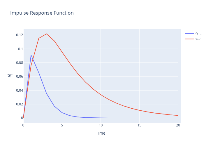
38.7.4. Step 4: compute impulse response functions#
To compute impulse response functions of \(k_t^i\), we use the impulse_response method of the
quantecon.LinearStateSpace class and plot outcomes.
xcoef, ycoef = lss.impulse_response(j=21)
data = np.array([xcoef])[0, :, 1, :]

fig = go.Figure(data=go.Scatter(y=data[:-1, 0], name=r'$e_{t+1}$'))
fig.add_trace(go.Scatter(y=data[1:, 1], name=r'$v_{t+1}$'))
fig.update_layout(title=r'Impulse Response Function',
                   xaxis_title='Time',
                   yaxis_title=r'$k^{i}_{t}$')
fig1 = fig
# Export to PNG file
Image(fig1.to_image(format="png", engine="kaleido"))
# fig1.show() will provide interactive plot when running
# notebook locally
/tmp/ipykernel_9302/651216215.py:11: DeprecationWarning:


Support for the 'engine' argument is deprecated and will be removed after September 2025.
Kaleido will be the only supported engine at that time.
38.7.5. Step 5: compute stationary covariance matrices and population regressions#
We compute stationary covariance matrices by
calling the stationary_distributions method of
the quantecon.LinearStateSpace class.
By appropriately decomposing the covariance matrix of the state vector, we obtain ingredients of pertinent population regression coefficients.
Define
where \(\Sigma_{11}\) is the covariance matrix of dependent variables and \(\Sigma_{22}\) is the covariance matrix of independent variables.
Regression coefficients are \(\beta=\Sigma_{21}\Sigma_{22}^{-1}\).
To verify an instance of a law of large numbers computation, we construct a long simulation of the state vector and for the resulting sample compute the ordinary least-squares estimator of \(\beta\) that we shall compare with corresponding population regression coefficients.
_, _, Σ_x, Σ_y, Σ_yx = lss.stationary_distributions()

Σ_11 = Σ_x[0, 0]
Σ_12 = Σ_x[0, 1:4]
Σ_21 = Σ_x[1:4, 0]
Σ_22 = Σ_x[1:4, 1:4]

reg_coeffs = Σ_12 @ np.linalg.inv(Σ_22)

print('Regression coefficients (e_t on k_t, P_t, \\tilde{\\theta_t})')
print('------------------------------')
print(r'k_t:', reg_coeffs[0])
print(r'\tilde{\theta_t}:', reg_coeffs[1])
print(r'P_t:', reg_coeffs[2])
Regression coefficients (e_t on k_t, P_t, \tilde{\theta_t})
------------------------------
k_t: -3.275556845219769
\tilde{\theta_t}: -0.9649461170475457
P_t: 0.9649461170475457
# Compute R squared
R_squared = reg_coeffs @ Σ_x[1:4, 1:4] @ reg_coeffs  / Σ_x[0, 0]
R_squared
np.float64(0.9649461170475461)
# Verify that the computed coefficients are close to least squares estimates
model = OLS(x[0], x[1:4].T)
reg_res = model.fit()
np.max(np.abs(reg_coeffs - reg_res.params)) < 1e-2
np.True_
# Verify that R_squared matches least squares estimate
np.abs(reg_res.rsquared - R_squared) < 1e-2
np.True_
# Verify that θ_t + e_t can be recovered
model = OLS(y[1], x[1:4].T)
reg_res = model.fit()
np.abs(reg_res.rsquared - 1.) < 1e-6
np.True_
38.8. Equilibrium with two noisy signals on \(\theta_t\)#
Steps 1, 4, and 5 are identical to those for the one-noisy-signal structure.
Step 2 requires a straightforward modification.
For step 3, we construct the following state-space representation so that we can get our hands on all of the random processes that we require in order to compute a regression of the noisy signal about \(\theta\) from the other industry that a firm receives directly in a pooling equilibrium against information that a firm would receive in Townsend’s original model.
For this purpose, we include equilibrium goods prices from both industries in the state vector:
A_ricc = np.array([[ρ]])
B_ricc = np.array([[np.sqrt(2)]])
R_ricc = np.array([[σ_e ** 2]])
Q_ricc = np.array([[σ_v ** 2]])
N_ricc = np.zeros((1, 1))
p = qe.solve_discrete_riccati(A_ricc, B_ricc, Q_ricc, R_ricc, N_ricc).item()

p_two = p  # Save for comparison later
# Verify that p = σ_v^2 + (pρ^2σ_e^2) / (2p + σ_e^2)
tol = 1e-12
np.abs(p - (σ_v ** 2 + p * ρ ** 2 * σ_e ** 2 / (2 * p + σ_e ** 2))) < tol
np.True_
κ = ρ * p / (2 * p + σ_e ** 2)
κ_prod = κ * σ_e ** 2 / p

κ_two = κ  # Save for comparison later

A_lss = np.array([[0., 0., 0., 0., 0., 0., 0., 0.],
                 [0., 0., 0., 0., 0., 0., 0., 0.],
                 [κ / (λ - ρ), κ / (λ - ρ), λ_tilde, -κ_prod / (λ - ρ), 0., 0., ρ / (λ - ρ), 0.],
                 [-κ, -κ, 0., κ_prod, 0., 0., 0., 1.],
                 [b * κ / (λ - ρ), b * κ / (λ - ρ), b * λ_tilde, -b * κ_prod / (λ - ρ), 0., 0., b * ρ / (λ - ρ) + ρ, 1.],
                 [b * κ / (λ - ρ), b * κ / (λ - ρ), b * λ_tilde, -b * κ_prod / (λ - ρ), 0., 0., b * ρ / (λ - ρ) + ρ, 1.],
                 [0., 0., 0., 0., 0., 0., ρ, 1.],
                 [0., 0., 0., 0., 0., 0., 0., 0.]])

C_lss = np.array([[σ_e, 0., 0.],
                 [0., σ_e, 0.],
                 [0., 0.,  0.],
                 [0., 0.,  0.],
                 [σ_e, 0., 0.],
                 [0., σ_e, 0.],
                 [0., 0., 0.],
                 [0., 0., σ_v]])

G_lss = np.array([[0., 0., 0., 0., 1., 0., 0., 0.],
                 [0., 0, 0, 0., 0., 1., 0., 0.],
                 [1., 0., 0., 0., 0., 0., 1., 0.],
                 [0., 1., 0., 0., 0., 0., 1., 0.],
                 [1., 0., 0., 0., 0., 0., 0., 0.],
                 [0., 1., 0., 0., 0., 0., 0., 0.]])
mu_0 = np.array([0., 0., 0., 0., 0., 0., 0., 0.])

lss = qe.LinearStateSpace(A_lss, C_lss, G_lss, mu_0=mu_0)
ts_length = 100_000
x, y = lss.simulate(ts_length, random_state=1)
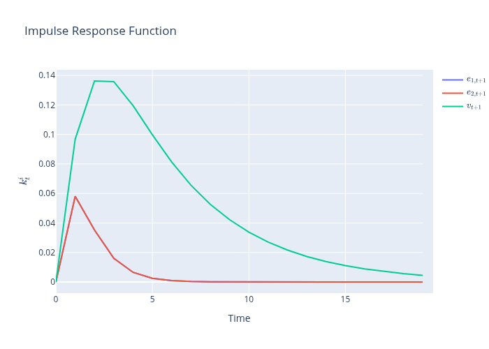
xcoef, ycoef = lss.impulse_response(j=20)
data = np.array([xcoef])[0, :, 2, :]

fig = go.Figure(data=go.Scatter(y=data[:-1, 0], name=r'$e_{1,t+1}$'))
fig.add_trace(go.Scatter(y=data[:-1, 1], name=r'$e_{2,t+1}$'))
fig.add_trace(go.Scatter(y=data[1:, 2], name=r'$v_{t+1}$'))
fig.update_layout(title=r'Impulse Response Function',
                   xaxis_title='Time',
                   yaxis_title=r'$k^{i}_{t}$')
fig2=fig
# Export to PNG file
Image(fig2.to_image(format="png"))
# fig2.show() will provide interactive plot when running
# notebook locally
_, _, Σ_x, Σ_y, Σ_yx = lss.stationary_distributions()

Σ_11 = Σ_x[1, 1]
Σ_12 = Σ_x[1, 2:5]
Σ_21 = Σ_x[2:5, 1]
Σ_22 = Σ_x[2:5, 2:5]

reg_coeffs = Σ_12 @ np.linalg.inv(Σ_22)

print('Regression coefficients (e_{2,t} on k_t, P^{1}_t, \\tilde{\\theta_t})')
print('------------------------------')
print(r'k_t:', reg_coeffs[0])
print(r'\tilde{\theta_t}:', reg_coeffs[1])
print(r'P_t:', reg_coeffs[2])
Regression coefficients (e_{2,t} on k_t, P^{1}_t, \tilde{\theta_t})
------------------------------
k_t: 0.0
\tilde{\theta_t}: 0.0
P_t: 0.0
# Compute R squared
R_squared = reg_coeffs @ Σ_x[2:5, 2:5] @ reg_coeffs  / Σ_x[1, 1]
R_squared
np.float64(0.0)
# Verify that the computed coefficients are close to least squares estimates
model = OLS(x[1], x[2:5].T)
reg_res = model.fit()
np.max(np.abs(reg_coeffs - reg_res.params)) < 1e-2
np.True_
# Verify that R_squared matches least squares estimate
np.abs(reg_res.rsquared - R_squared) < 1e-2
np.True_
_, _, Σ_x, Σ_y, Σ_yx = lss.stationary_distributions()

Σ_11 = Σ_x[1, 1]
Σ_12 = Σ_x[1, 2:6]
Σ_21 = Σ_x[2:6, 1]
Σ_22 = Σ_x[2:6, 2:6]

reg_coeffs = Σ_12 @ np.linalg.inv(Σ_22)

print('Regression coefficients (e_{2,t} on k_t, P^{1}_t, P^{2}_t, \\tilde{\\theta_t})')
print('------------------------------')
print(r'k_t:', reg_coeffs[0])
print(r'\tilde{\theta_t}:', reg_coeffs[1])
print(r'P^{1}_t:', reg_coeffs[2])
print(r'P^{2}_t:', reg_coeffs[3])
Regression coefficients (e_{2,t} on k_t, P^{1}_t, P^{2}_t, \tilde{\theta_t})
------------------------------
k_t: -3.137358917103563
\tilde{\theta_t}: -0.9242343967443674
P^{1}_t: -0.03788280162781599
P^{2}_t: 0.9621171983721835
# Compute R squared
R_squared = reg_coeffs @ Σ_x[2:6, 2:6] @ reg_coeffs  / Σ_x[1, 1]
R_squared
np.float64(0.9621171983721837)
38.9. Key step#
Now we come to the key step for verifying that equilibrium outcomes for prices and quantities are identical in the pooling equilibrium original model that led Townsend to deduce an infinite-dimensional state space.
We accomplish this by computing a population linear least squares regression of the noisy signal that firms in the other industry receive in a pooling equilibrium on time \(t\) information that a firm would receive in Townsend’s original model.
Let’s compute the regression and stare at the \(R^2\):
# Verify that θ_t + e^{2}_t can be recovered

# θ_t + e^{2}_t on k^{i}_t, P^{1}_t, P^{2}_t, \\tilde{\\theta_t}


model = OLS(y[1], x[2:6].T)
reg_res = model.fit()
np.abs(reg_res.rsquared - 1.) < 1e-6
np.True_
reg_res.rsquared
np.float64(1.0)
The \(R^2\) in this regression equals \(1\).
That verifies that a firm’s information set in Townsend’s original model equals its information set in a pooling equilibrium.
Therefore, equilibrium prices and quantities in Townsend’s original model equal those in a pooling equilibrium.
38.10. An observed common shock benchmark#
For purposes of comparison, it is useful to construct a model in which demand disturbance in both industries still both share have a common persistent component \(\theta_t\), but in which the persistent component \(\theta\) is observed each period.
In this case, firms share the same information immediately and have no need to deploy signal-extraction techniques.
Thus, consider a version of our model in which histories of both \(\epsilon_t^i\) and \(\theta_t\) are observed by a representative firm.
In this case, the firm’s optimal decision rule is described by
where \(\hat \theta_{t+1} = E_t \theta_{t+1}\) is given by
Thus, the firm’s decision rule can be expressed
Consequently, when a history \(\theta_s, s \leq t\) is observed without noise, the following state space system prevails:
where \(z_{t,t+1} \) is a scalar iid standardized Gaussian process.
As usual, the system can be written as
In order once again to use the quantecon class quantecon.LinearStateSpace, let’s form pertinent state-space matrices
Ao_lss = np.array([[ρ, 0.],
                 [ρ / (λ - ρ), λ_tilde]])

Co_lss = np.array([[σ_v], [0.]])

Go_lss = np.identity(2)
muo_0 = np.array([0., 0.])

lsso = qe.LinearStateSpace(Ao_lss, Co_lss, Go_lss, mu_0=muo_0)
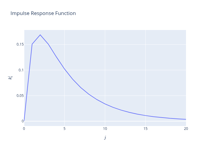
Now let’s form and plot an impulse response function of \(k_t^i\) to shocks \(v_t\) to \(\theta_{t+1}\)
xcoef, ycoef = lsso.impulse_response(j=21)
data = np.array([ycoef])[0, :, 1, :]

fig = go.Figure(data=go.Scatter(y=data[:-1, 0], name=r'$z_{t+1}$'))
fig.update_layout(title=r'Impulse Response Function',
                   xaxis_title= r'lag $j$',
                   yaxis_title=r'$k^{i}_{t}$')
fig3 = fig
# Export to PNG file
Image(fig3.to_image(format="png"))
# fig1.show() will provide interactive plot when running
# notebook locally
38.11. Comparison of all signal structures#
It is enlightening side by side to plot impulse response functions for capital for the two noisy-signal information structures and the noiseless signal on \(\theta\) that we have just presented.
Please remember that the two-signal structure corresponds to the pooling equilibrium and also Townsend’s original model.
fig_comb = go.Figure(data=[
                        *fig1.data,
                        *fig2.update_traces(xaxis='x2', yaxis='y2').data,
                        *fig3.update_traces(xaxis='x3', yaxis='y3').data
                    ]).set_subplots(1, 3,
                           subplot_titles=("One noisy-signal",
                                           "Two noisy-signal",
                                           "No Noise"),
                           horizontal_spacing=0.02,
                           shared_yaxes=True)
# Export to PNG file
Image(fig_comb.to_image(format="png"))
# fig_comb.show() # will provide interactive plot when running
# notebook locally
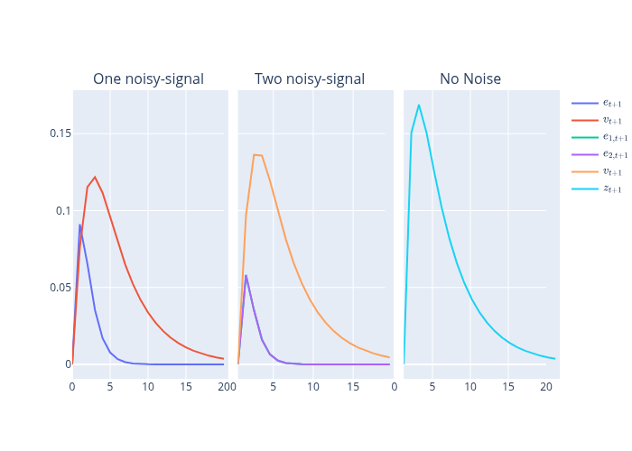
The three panels in the graph above show that
responses of \( k_t^i \) to shocks \( v_t \) to the hidden Markov demand state \( \theta_t \) process are largest in the no-noisy-signal structure in which the firm observes \(\theta_t\) at time \(t\)
responses of \( k_t^i \) to shocks \( v_t \) to the hidden Markov demand state \( \theta_t \) process are smaller in the two-noisy-signal structure
responses of \( k_t^i \) to shocks \( v_t \) to the hidden Markov demand state \( \theta_t \) process are smallest in the one-noisy-signal structure
With respect to the iid demand shocks \(e_t\) the graphs show that
responses of \( k_t^i \) to shocks \( e_t \) to the hidden Markov demand state \( \theta_t \) process are smallest (i.e., nonexistent) in the no-noisy-signal structure in which the firm observes \(\theta_t\) at time \(t\)
responses of \( k_t^i \) to shocks \( e_t \) to the hidden Markov demand state \( \theta_t \) process are larger in the two-noisy-signal structure
responses of \( k_t^i \) to idiosyncratic own-market noise-shocks \( e_t \) are largest in the one-noisy-signal structure
Among other things, these findings indicate that time series correlations and coherences between outputs in the two industries are higher in the two-noisy-signals or pooling model than they are in the one-noisy signal model.
The enhanced influence of the shocks \( v_t \) to the hidden Markov demand state \( \theta_t \) process that emerges from the two-noisy-signal model relative to the one-noisy-signal model is a symptom of a lower equilibrium hidden-state reconstruction error variance in the two-signal model:
display(Latex('$\\textbf{Reconstruction error variances}$'))
display(Latex(f'One-noise structure: {round(p_one, 6)}'))
display(Latex(f'Two-noise structure: {round(p_two, 6)}'))
Kalman gains for the two structures are
display(Latex('$\\textbf{Kalman Gains}$'))
display(Latex(f'One noisy-signal structure: {round(κ_one, 6)}'))
display(Latex(f'Two noisy-signals structure: {round(κ_two, 6)}'))
Another lesson that comes from the preceding three-panel graph is that the presence of iid noise \(\epsilon_t^i\) in industry \(i\) generates a response in \(k_t^{-i}\) in the two-noisy-signal structure, but not in the one-noisy-signal structure.
38.12. Notes on history of the problem#
To truncate what he saw as an intractable, infinite dimensional state space, Townsend constructed an approximating model in which the common hidden Markov demand shock is revealed to all firms after a fixed number of periods.
Thus,
Townsend wanted to assume that at time \( t \) firms in industry \( i \) observe \( k_t^i, Y_t^i, P_t^i, (P^{-i})^t \), where \( (P^{-i})^t \) is the history of prices in the other market up to time \( t \).
Because that turned out to be too challenging, Townsend made a sensible alternative assumption that eased his calculations: that after a large number \( S \) of periods, firms in industry \( i \) observe the hidden Markov component of the demand shock \( \theta_{t-S} \).
Townsend argued that the more manageable model could do a good job of approximating the intractable model in which the Markov component of the demand shock remains unobserved for ever.
By applying technical machinery of [Pearlman et al., 1986], [Pearlman and Sargent, 2005] showed that there is a recursive representation of the equilibrium of the perpetually and symmetrically uninformed model that Townsend wanted to solve [Townsend, 1983].
A reader of [Pearlman and Sargent, 2005] will notice that their representation of the equilibrium of Townsend’s model exactly matches that of the pooling equilibrium presented here.
We have structured our notation in this lecture to faciliate comparison of the pooling equilibrium constructed here with the equilibrium of Townsend’s model reported in [Pearlman and Sargent, 2005].
The computational method of [Pearlman and Sargent, 2005] is recursive: it enlists the Kalman filter and invariant subspace methods for solving systems of Euler equations [5] .
As [Singleton, 1987], [Kasa, 2000], and [Sargent, 1991] also found, the equilibrium is fully revealing: observed prices tell participants in industry \( i \) all of the information held by participants in market \( -i \) (\( -i \) means not \( i \)).
This means that higher-order beliefs play no role: observing equilibrium prices in effect lets decision makers pool their information sets [6] .
The disappearance of higher order beliefs means that decision makers in this model do not really face a problem of forecasting the forecasts of others.
Because those forecasts are the same as their own, they know them.
38.12.1. Further historical remarks#
Sargent [Sargent, 1991] proposed a way to compute an equilibrium without making Townsend’s approximation.
Extending the reasoning of [Muth, 1960], Sargent noticed that it is possible to summarize the relevant history with a low dimensional object, namely, a small number of current and lagged forecasting errors.
Positing an equilibrium in a space of perceived laws of motion for endogenous variables that takes the form of a vector autoregressive, moving average, Sargent described an equilibrium as a fixed point of a mapping from the perceived law of motion to the actual law of motion of that form.
Sargent worked in the time domain and proceeded to guess and verify the appropriate orders of the autoregressive and moving average pieces of the equilibrium representation.
By working in the frequency domain [Kasa, 2000] showed how to discover the appropriate orders of the autoregressive and moving average parts, and also how to compute an equilibrium.
The [Pearlman and Sargent, 2005] recursive computational method, which stays in the time domain, also discovered appropriate orders of the autoregressive and moving average pieces.
In addition, by displaying equilibrium representations in the form of [Pearlman et al., 1986], [Pearlman and Sargent, 2005] showed how the moving average piece is linked to the innovation process of the hidden persistent component of the demand shock.
That scalar innovation process is the additional state variable contributed by the problem of extracting a signal from equilibrium prices that decision makers face in Townsend’s model.