4. Discrete State Dynamic Programming #

Contents

Discrete State Dynamic Programming

In addition to what’s in Anaconda, this lecture will need the following libraries:

!pip install --upgrade quantecon

4.1. Overview #

In this lecture we discuss a family of dynamic programming problems with the following features:

a discrete state space and discrete choices (actions)
an infinite horizon
discounted rewards
Markov state transitions

We call such problems discrete dynamic programs or discrete DPs.

Discrete DPs are the workhorses in much of modern quantitative economics, including

monetary economics
search and labor economics
household savings and consumption theory
investment theory
asset pricing
industrial organization, etc.

When a given model is not inherently discrete, it is common to replace it with a discretized version in order to use discrete DP techniques.

This lecture covers

the theory of dynamic programming in a discrete setting, plus examples and applications
a powerful set of routines for solving discrete DPs from the QuantEcon code library

Let’s start with some imports:

import numpy as np
import matplotlib.pyplot as plt
%matplotlib inline
import quantecon as qe
import scipy.sparse as sparse
from quantecon import compute_fixed_point
from quantecon.markov import DiscreteDP

4.1.1. How to Read this Lecture#

We use dynamic programming many applied lectures, such as

The shortest path lecture
The McCall search model lecture

The objective of this lecture is to provide a more systematic and theoretical treatment, including algorithms and implementation while focusing on the discrete case.

4.1.2. Code#

Among other things, it offers

a flexible, well-designed interface
multiple solution methods, including value function and policy function iteration
high-speed operations via carefully optimized JIT-compiled functions
the ability to scale to large problems by minimizing vectorized operators and allowing operations on sparse matrices

JIT compilation relies on Numba, which should work seamlessly if you are using Anaconda as suggested.

4.1.3. References#

For background reading on dynamic programming and additional applications, see, for example,

[LS18]
[HLL96], section 3.5
[Put05]
[SLP89]
[Rus96]
[MF02]
EDTC, chapter 5

4.2. Discrete DPs #

Loosely speaking, a discrete DP is a maximization problem with an objective function of the form

(4.1)#\[\mathbb{E} \sum_{t = 0}^{\infty} \beta^t r(s_t, a_t)\]

where

\(s_t\) is the state variable
\(a_t\) is the action
\(\beta\) is a discount factor
\(r(s_t, a_t)\) is interpreted as a current reward when the state is \(s_t\) and the action chosen is \(a_t\)

Each pair \((s_t, a_t)\) pins down transition probabilities \(Q(s_t, a_t, s_{t+1})\) for the next period state \(s_{t+1}\).

Thus, actions influence not only current rewards but also the future time path of the state.

The essence of dynamic programming problems is to trade off current rewards vs favorable positioning of the future state (modulo randomness).

Examples:

consuming today vs saving and accumulating assets
accepting a job offer today vs seeking a better one in the future
exercising an option now vs waiting

4.2.1. Policies#

The most fruitful way to think about solutions to discrete DP problems is to compare policies.

In general, a policy is a randomized map from past actions and states to current action.

In the setting formalized below, it suffices to consider so-called stationary Markov policies, which consider only the current state.

In particular, a stationary Markov policy is a map \(\sigma\) from states to actions

\(a_t = \sigma(s_t)\) indicates that \(a_t\) is the action to be taken in state \(s_t\)

It is known that, for any arbitrary policy, there exists a stationary Markov policy that dominates it at least weakly.

See section 5.5 of [Put05] for discussion and proofs.

In what follows, stationary Markov policies are referred to simply as policies.

The aim is to find an optimal policy, in the sense of one that maximizes (4.1).

Let’s now step through these ideas more carefully.

4.2.2. Formal Definition#

Formally, a discrete dynamic program consists of the following components:

A finite set of states \(S = \{0, \ldots, n-1\}\).
A finite set of feasible actions \(A(s)\) for each state \(s \in S\), and a corresponding set of feasible state-action pairs.

\[ \mathit{SA} := \{(s, a) \mid s \in S, \; a \in A(s)\} \]
A reward function \(r\colon \mathit{SA} \to \mathbb{R}\).
A transition probability function \(Q\colon \mathit{SA} \to \Delta(S)\), where \(\Delta(S)\) is the set of probability distributions over \(S\).
A discount factor \(\beta \in [0, 1)\).

We also use the notation \(A := \bigcup_{s \in S} A(s) = \{0, \ldots, m-1\}\) and call this set the action space.

A policy is a function \(\sigma\colon S \to A\).

A policy is called feasible if it satisfies \(\sigma(s) \in A(s)\) for all \(s \in S\).

Denote the set of all feasible policies by \(\Sigma\).

If a decision-maker uses a policy \(\sigma \in \Sigma\), then

the current reward at time \(t\) is \(r(s_t, \sigma(s_t))\)
the probability that \(s_{t+1} = s'\) is \(Q(s_t, \sigma(s_t), s')\)

For each \(\sigma \in \Sigma\), define

\(r_{\sigma}\) by \(r_{\sigma}(s) := r(s, \sigma(s))\))
\(Q_{\sigma}\) by \(Q_{\sigma}(s, s') := Q(s, \sigma(s), s')\)

Notice that \(Q_\sigma\) is a stochastic matrix on \(S\).

It gives transition probabilities of the controlled chain when we follow policy \(\sigma\).

If we think of \(r_\sigma\) as a column vector, then so is \(Q_\sigma^t r_\sigma\), and the \(s\)-th row of the latter has the interpretation

(4.2)#\[(Q_\sigma^t r_\sigma)(s) = \mathbb E [ r(s_t, \sigma(s_t)) \mid s_0 = s ] \quad \text{when } \{s_t\} \sim Q_\sigma\]

Comments

\(\{s_t\} \sim Q_\sigma\) means that the state is generated by stochastic matrix \(Q_\sigma\).
See this discussion on computing expectations of Markov chains for an explanation of the expression in (4.2).

Notice that we’re not really distinguishing between functions from \(S\) to \(\mathbb R\) and vectors in \(\mathbb R^n\).

This is natural because they are in one to one correspondence.

4.2.3. Value and Optimality#

Let \(v_{\sigma}(s)\) denote the discounted sum of expected reward flows from policy \(\sigma\) when the initial state is \(s\).

To calculate this quantity we pass the expectation through the sum in (4.1) and use (4.2) to get

\[ v_{\sigma}(s) = \sum_{t=0}^{\infty} \beta^t (Q_{\sigma}^t r_{\sigma})(s) \qquad (s \in S) \]

This function is called the policy value function for the policy \(\sigma\).

The optimal value function, or simply value function, is the function \(v^*\colon S \to \mathbb{R}\) defined by

\[ v^*(s) = \max_{\sigma \in \Sigma} v_{\sigma}(s) \qquad (s \in S) \]

(We can use max rather than sup here because the domain is a finite set)

A policy \(\sigma \in \Sigma\) is called optimal if \(v_{\sigma}(s) = v^*(s)\) for all \(s \in S\).

Given any \(w \colon S \to \mathbb R\), a policy \(\sigma \in \Sigma\) is called \(w\)-greedy if

\[ \sigma(s) \in \operatorname*{arg\,max}_{a \in A(s)} \left\{ r(s, a) + \beta \sum_{s' \in S} w(s') Q(s, a, s') \right\} \qquad (s \in S) \]

As discussed in detail below, optimal policies are precisely those that are \(v^*\)-greedy.

4.2.4. Two Operators#

It is useful to define the following operators:

The Bellman operator \(T\colon \mathbb{R}^S \to \mathbb{R}^S\) is defined by

\[ (T v)(s) = \max_{a \in A(s)} \left\{ r(s, a) + \beta \sum_{s' \in S} v(s') Q(s, a, s') \right\} \qquad (s \in S) \]

For any policy function \(\sigma \in \Sigma\), the operator \(T_{\sigma}\colon \mathbb{R}^S \to \mathbb{R}^S\) is defined by

\[ (T_{\sigma} v)(s) = r(s, \sigma(s)) + \beta \sum_{s' \in S} v(s') Q(s, \sigma(s), s') \qquad (s \in S) \]

This can be written more succinctly in operator notation as

\[ T_{\sigma} v = r_{\sigma} + \beta Q_{\sigma} v \]

The two operators are both monotone

\(v \leq w\) implies \(Tv \leq Tw\) pointwise on \(S\), and similarly for \(T_\sigma\)

They are also contraction mappings with modulus \(\beta\)

\(\lVert Tv - Tw \rVert \leq \beta \lVert v - w \rVert\) and similarly for \(T_\sigma\), where \(\lVert \cdot\rVert\) is the max norm

For any policy \(\sigma\), its value \(v_{\sigma}\) is the unique fixed point of \(T_{\sigma}\).

For proofs of these results and those in the next section, see, for example, EDTC, chapter 10.

4.2.5. The Bellman Equation and the Principle of Optimality#

The main principle of the theory of dynamic programming is that

the optimal value function \(v^*\) is a unique solution to the Bellman equation

\[ v(s) = \max_{a \in A(s)} \left\{ r(s, a) + \beta \sum_{s' \in S} v(s') Q(s, a, s') \right\} \qquad (s \in S) \]

or in other words, \(v^*\) is the unique fixed point of \(T\), and

\(\sigma^*\) is an optimal policy function if and only if it is \(v^*\)-greedy

By the definition of greedy policies given above, this means that

\[ \sigma^*(s) \in \operatorname*{arg\,max}_{a \in A(s)} \left\{ r(s, a) + \beta \sum_{s' \in S} v^*(s') Q(s, a, s') \right\} \qquad (s \in S) \]

4.3. Solving Discrete DPs #

Now that the theory has been set out, let’s turn to solution methods.

The code for solving discrete DPs is available in ddp.py from the QuantEcon.py code library.

It implements the three most important solution methods for discrete dynamic programs, namely

value function iteration
policy function iteration
modified policy function iteration

Let’s briefly review these algorithms and their implementation.

4.3.1. Value Function Iteration#

Perhaps the most familiar method for solving all manner of dynamic programs is value function iteration.

This algorithm uses the fact that the Bellman operator \(T\) is a contraction mapping with fixed point \(v^*\).

Hence, iterative application of \(T\) to any initial function \(v^0 \colon S \to \mathbb R\) converges to \(v^*\).

The details of the algorithm can be found in the appendix.

4.3.2. Policy Function Iteration#

This routine, also known as Howard’s policy improvement algorithm, exploits more closely the particular structure of a discrete DP problem.

Each iteration consists of

A policy evaluation step that computes the value \(v_{\sigma}\) of a policy \(\sigma\) by solving the linear equation \(v = T_{\sigma} v\).
A policy improvement step that computes a \(v_{\sigma}\)-greedy policy.

In the current setting, policy iteration computes an exact optimal policy in finitely many iterations.

See theorem 10.2.6 of EDTC for a proof.

The details of the algorithm can be found in the appendix.

4.3.3. Modified Policy Function Iteration#

Modified policy iteration replaces the policy evaluation step in policy iteration with “partial policy evaluation”.

The latter computes an approximation to the value of a policy \(\sigma\) by iterating \(T_{\sigma}\) for a specified number of times.

This approach can be useful when the state space is very large and the linear system in the policy evaluation step of policy iteration is correspondingly difficult to solve.

The details of the algorithm can be found in the appendix.

4.4. Example: A Growth Model #

Let’s consider a simple consumption-saving model.

A single household either consumes or stores its own output of a single consumption good.

The household starts each period with current stock \(s\).

Next, the household chooses a quantity \(a\) to store and consumes \(c = s - a\)

Storage is limited by a global upper bound \(M\).
Flow utility is \(u(c) = c^{\alpha}\).

Output is drawn from a discrete uniform distribution on \(\{0, \ldots, B\}\).

The next period stock is therefore

\[ s' = a + U \quad \text{where} \quad U \sim U[0, \ldots, B] \]

The discount factor is \(\beta \in [0, 1)\).

4.4.1. Discrete DP Representation#

We want to represent this model in the format of a discrete dynamic program.

To this end, we take

the state variable to be the stock \(s\)
the state space to be \(S = \{0, \ldots, M + B\}\)
- hence \(n = M + B + 1\)
the action to be the storage quantity \(a\)
the set of feasible actions at \(s\) to be \(A(s) = \{0, \ldots, \min\{s, M\}\}\)
- hence \(A = \{0, \ldots, M\}\) and \(m = M + 1\)
the reward function to be \(r(s, a) = u(s - a)\)
the transition probabilities to be

(4.3)#\[\begin{split}Q(s, a, s') := \begin{cases} \frac{1}{B + 1} & \text{if } a \leq s' \leq a + B \\ 0 & \text{ otherwise} \end{cases}\end{split}\]

4.4.2. Defining a DiscreteDP Instance#

This information will be used to create an instance of DiscreteDP by passing the following information

An \(n \times m\) reward array \(R\).
An \(n \times m \times n\) transition probability array \(Q\).
A discount factor \(\beta\).

For \(R\) we set \(R[s, a] = u(s - a)\) if \(a \leq s\) and \(-\infty\) otherwise.

For \(Q\) we follow the rule in (4.3).

Note

The feasibility constraint is embedded into \(R\) by setting \(R[s, a] = -\infty\) for \(a \notin A(s)\).
Probability distributions for \((s, a)\) with \(a \notin A(s)\) can be arbitrary.

The following code sets up these objects for us

class SimpleOG:

    def __init__(self, B=10, M=5, α=0.5, β=0.9):
        """
        Set up R, Q and β, the three elements that define an instance of
        the DiscreteDP class.
        """

        self.B, self.M, self.α, self.β  = B, M, α, β
        self.n = B + M + 1
        self.m = M + 1

        self.R = np.empty((self.n, self.m))
        self.Q = np.zeros((self.n, self.m, self.n))

        self.populate_Q()
        self.populate_R()

    def u(self, c):
        return c**self.α

    def populate_R(self):
        """
        Populate the R matrix, with R[s, a] = -np.inf for infeasible
        state-action pairs.
        """
        for s in range(self.n):
            for a in range(self.m):
                self.R[s, a] = self.u(s - a) if a <= s else -np.inf

    def populate_Q(self):
        """
        Populate the Q matrix by setting

            Q[s, a, s'] = 1 / (1 + B) if a <= s' <= a + B

        and zero otherwise.
        """

        for a in range(self.m):
            self.Q[:, a, a:(a + self.B + 1)] = 1.0 / (self.B + 1)

Let’s run this code and create an instance of SimpleOG.

g = SimpleOG()  # Use default parameters

Instances of DiscreteDP are created using the signature DiscreteDP(R, Q, β).

Let’s create an instance using the objects stored in g

ddp = qe.markov.DiscreteDP(g.R, g.Q, g.β)

Now that we have an instance ddp of DiscreteDP we can solve it as follows

results = ddp.solve(method='policy_iteration')

Let’s see what we’ve got here

dir(results)

['max_iter', 'mc', 'method', 'num_iter', 'sigma', 'v']

(In IPython version 4.0 and above you can also type results. and hit the tab key)

The most important attributes are v, the value function, and σ, the optimal policy

results.v

array([19.01740222, 20.01740222, 20.43161578, 20.74945302, 21.04078099,
       21.30873018, 21.54479816, 21.76928181, 21.98270358, 22.18824323,
       22.3845048 , 22.57807736, 22.76109127, 22.94376708, 23.11533996,
       23.27761762])

results.sigma

array([0, 0, 0, 0, 1, 1, 1, 2, 2, 3, 3, 4, 5, 5, 5, 5])

Since we’ve used policy iteration, these results will be exact unless we hit the iteration bound max_iter.

Let’s make sure this didn’t happen

results.max_iter

results.num_iter

Another interesting object is results.mc, which is the controlled chain defined by \(Q_{\sigma^*}\), where \(\sigma^*\) is the optimal policy.

In other words, it gives the dynamics of the state when the agent follows the optimal policy.

Since this object is an instance of MarkovChain from QuantEcon.py (see this lecture for more discussion), we can easily simulate it, compute its stationary distribution and so on.

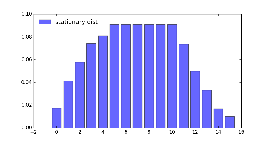
results.mc.stationary_distributions

array([[0.01732187, 0.04121063, 0.05773956, 0.07426848, 0.08095823,
        0.09090909, 0.09090909, 0.09090909, 0.09090909, 0.09090909,
        0.09090909, 0.07358722, 0.04969846, 0.03316953, 0.01664061,
        0.00995086]])

Here’s the same information in a bar graph

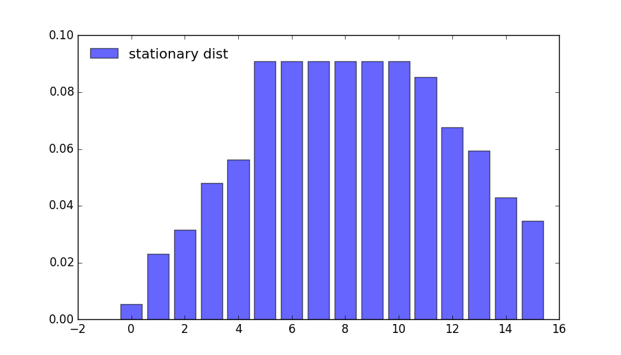
What happens if the agent is more patient?

ddp = qe.markov.DiscreteDP(g.R, g.Q, 0.99)  # Increase β to 0.99
results = ddp.solve(method='policy_iteration')
results.mc.stationary_distributions

array([[0.00546913, 0.02321342, 0.03147788, 0.04800681, 0.05627127,
        0.09090909, 0.09090909, 0.09090909, 0.09090909, 0.09090909,
        0.09090909, 0.08543996, 0.06769567, 0.05943121, 0.04290228,
        0.03463782]])

If we look at the bar graph we can see the rightward shift in probability mass

4.4.3. State-Action Pair Formulation#

The DiscreteDP class in fact, provides a second interface to set up an instance.

One of the advantages of this alternative set up is that it permits the use of a sparse matrix for Q.

(An example of using sparse matrices is given in the exercises below)

The call signature of the second formulation is DiscreteDP(R, Q, β, s_indices, a_indices) where

s_indices and a_indices are arrays of equal length L enumerating all feasible state-action pairs
R is an array of length L giving corresponding rewards
Q is an L x n transition probability array

Here’s how we could set up these objects for the preceding example

B, M, α, β = 10, 5, 0.5, 0.9
n = B + M + 1
m = M + 1

def u(c):
    return c**α

s_indices = []
a_indices = []
Q = []
R = []
b = 1.0 / (B + 1)

for s in range(n):
    for a in range(min(M, s) + 1):  # All feasible a at this s
        s_indices.append(s)
        a_indices.append(a)
        q = np.zeros(n)
        q[a:(a + B + 1)] = b        # b on these values, otherwise 0
        Q.append(q)
        R.append(u(s - a))

ddp = qe.markov.DiscreteDP(R, Q, β, s_indices, a_indices)

For larger problems, you might need to write this code more efficiently by vectorizing or using Numba.

4.5. Exercises #

In the stochastic optimal growth lecture from our introductory lecture series, we solve a benchmark model that has an analytical solution.

The exercise is to replicate this solution using DiscreteDP.

4.6. Solutions #

4.6.1. Setup#

Details of the model can be found in the lecture on optimal growth.

We let \(f(k) = k^{\alpha}\) with \(\alpha = 0.65\), \(u(c) = \log c\), and \(\beta = 0.95\)

α = 0.65
f = lambda k: k**α
u = np.log
β = 0.95

Here we want to solve a finite state version of the continuous state model above.

We discretize the state space into a grid of size grid_size=500, from \(10^{-6}\) to grid_max=2

grid_max = 2
grid_size = 500
grid = np.linspace(1e-6, grid_max, grid_size)

We choose the action to be the amount of capital to save for the next period (the state is the capital stock at the beginning of the period).

Thus the state indices and the action indices are both 0, …, grid_size-1.

Action (indexed by) a is feasible at state (indexed by) s if and only if grid[a] < f([grid[s]) (zero consumption is not allowed because of the log utility).

Thus the Bellman equation is:

\[ v(k) = \max_{0 < k' < f(k)} u(f(k) - k') + \beta v(k'), \]

where \(k'\) is the capital stock in the next period.

The transition probability array Q will be highly sparse (in fact it is degenerate as the model is deterministic), so we formulate the problem with state-action pairs, to represent Q in scipy sparse matrix format.

We first construct indices for state-action pairs:

# Consumption matrix, with nonpositive consumption included
C = f(grid).reshape(grid_size, 1) - grid.reshape(1, grid_size)

# State-action indices
s_indices, a_indices = np.where(C > 0)

# Number of state-action pairs
L = len(s_indices)

print(L)
print(s_indices)
print(a_indices)

118841
[  0   1   1 ... 499 499 499]
[  0   0   1 ... 389 390 391]

Reward vector R (of length L):

R = u(C[s_indices, a_indices])

(Degenerate) transition probability matrix Q (of shape (L, grid_size)), where we choose the scipy.sparse.lil_matrix format, while any format will do (internally it will be converted to the csr format):

Q = sparse.lil_matrix((L, grid_size))
Q[np.arange(L), a_indices] = 1

(If you are familiar with the data structure of scipy.sparse.csr_matrix, the following is the most efficient way to create the Q matrix in the current case)

# data = np.ones(L)
# indptr = np.arange(L+1)
# Q = sparse.csr_matrix((data, a_indices, indptr), shape=(L, grid_size))

Discrete growth model:

ddp = DiscreteDP(R, Q, β, s_indices, a_indices)

Notes

Here we intensively vectorized the operations on arrays to simplify the code.

As noted, however, vectorization is memory consumptive, and it can be prohibitively so for grids with large size.

4.6.2. Solving the Model#

Solve the dynamic optimization problem:

res = ddp.solve(method='policy_iteration')
v, σ, num_iter = res.v, res.sigma, res.num_iter
num_iter

Note that sigma contains the indices of the optimal capital stocks to save for the next period. The following translates sigma to the corresponding consumption vector.

# Optimal consumption in the discrete version
c = f(grid) - grid[σ]

# Exact solution of the continuous version
ab = α * β
c1 = (np.log(1 - ab) + np.log(ab) * ab / (1 - ab)) / (1 - β)
c2 = α / (1 - ab)

def v_star(k):
    return c1 + c2 * np.log(k)

def c_star(k):
    return (1 - ab) * k**α

Let us compare the solution of the discrete model with that of the original continuous model

fig, ax = plt.subplots(1, 2, figsize=(14, 4))
ax[0].set_ylim(-40, -32)
ax[0].set_xlim(grid[0], grid[-1])
ax[1].set_xlim(grid[0], grid[-1])

lb0 = 'discrete value function'
ax[0].plot(grid, v, lw=2, alpha=0.6, label=lb0)

lb0 = 'continuous value function'
ax[0].plot(grid, v_star(grid), 'k-', lw=1.5, alpha=0.8, label=lb0)
ax[0].legend(loc='upper left')

lb1 = 'discrete optimal consumption'
ax[1].plot(grid, c, 'b-', lw=2, alpha=0.6, label=lb1)

lb1 = 'continuous optimal consumption'
ax[1].plot(grid, c_star(grid), 'k-', lw=1.5, alpha=0.8, label=lb1)
ax[1].legend(loc='upper left')
plt.show()

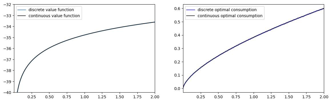
_images/6575f4766a36b7c84572f68ad2580d52f510443c8a38cd766a74a11b8450c43a.png

The outcomes appear very close to those of the continuous version.

Except for the “boundary” point, the value functions are very close:

np.abs(v - v_star(grid)).max()

121.49819147053378

np.abs(v - v_star(grid))[1:].max()

0.012681735127500815

The optimal consumption functions are close as well:

np.abs(c - c_star(grid)).max()

0.003826523100010082

In fact, the optimal consumption obtained in the discrete version is not really monotone, but the decrements are quite small:

diff = np.diff(c)
(diff >= 0).all()

False

dec_ind = np.where(diff < 0)[0]
len(dec_ind)

np.abs(diff[dec_ind]).max()

0.001961853339766839

The value function is monotone:

(np.diff(v) > 0).all()

True

4.6.3. Comparison of the Solution Methods#

Let us solve the problem with the other two methods.

4.6.3.1. Value Iteration#

ddp.epsilon = 1e-4
ddp.max_iter = 500
res1 = ddp.solve(method='value_iteration')
res1.num_iter

np.array_equal(σ, res1.sigma)

True

4.6.3.2. Modified Policy Iteration#

res2 = ddp.solve(method='modified_policy_iteration')
res2.num_iter

np.array_equal(σ, res2.sigma)

True

4.6.3.3. Speed Comparison#

%timeit ddp.solve(method='value_iteration')
%timeit ddp.solve(method='policy_iteration')
%timeit ddp.solve(method='modified_policy_iteration')

91.5 ms ± 74.3 µs per loop (mean ± std. dev. of 7 runs, 10 loops each)

9.34 ms ± 26.2 µs per loop (mean ± std. dev. of 7 runs, 100 loops each)

10.8 ms ± 15.8 µs per loop (mean ± std. dev. of 7 runs, 100 loops each)

As is often the case, policy iteration and modified policy iteration are much faster than value iteration.

4.6.4. Replication of the Figures#

Using DiscreteDP we replicate the figures shown in the lecture.

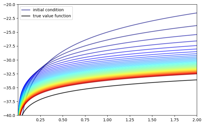
4.6.4.1. Convergence of Value Iteration#

Let us first visualize the convergence of the value iteration algorithm as in the lecture, where we use ddp.bellman_operator implemented as a method of DiscreteDP

w = 5 * np.log(grid) - 25  # Initial condition
n = 35
fig, ax = plt.subplots(figsize=(8,5))
ax.set_ylim(-40, -20)
ax.set_xlim(np.min(grid), np.max(grid))
lb = 'initial condition'
ax.plot(grid, w, color=plt.cm.jet(0), lw=2, alpha=0.6, label=lb)
for i in range(n):
    w = ddp.bellman_operator(w)
    ax.plot(grid, w, color=plt.cm.jet(i / n), lw=2, alpha=0.6)
lb = 'true value function'
ax.plot(grid, v_star(grid), 'k-', lw=2, alpha=0.8, label=lb)
ax.legend(loc='upper left')

plt.show()

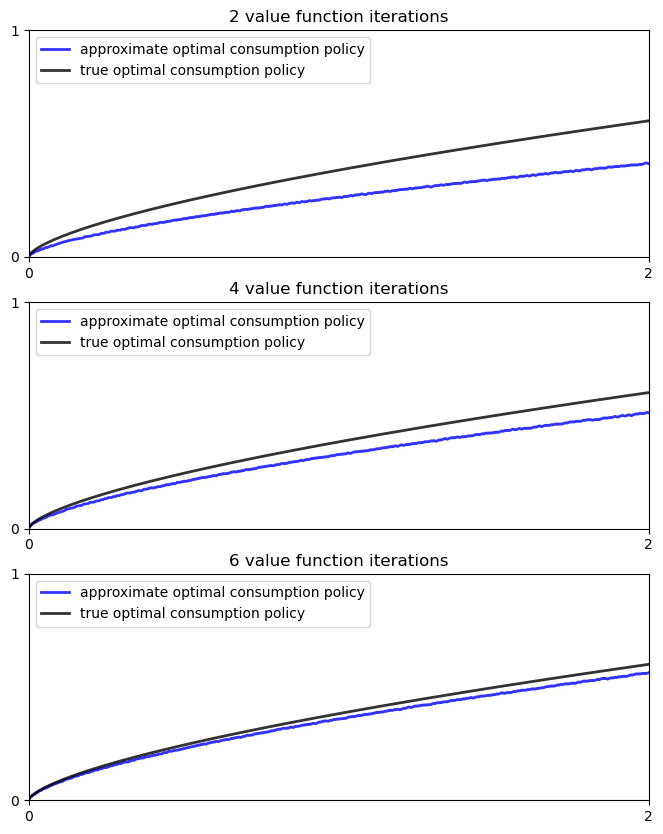
_images/f8efd9e1c2b5520523d037cfe56c8cbecd9ee817dc4f7842ecc014270fae3d2e.png

We next plot the consumption policies along with the value iteration

w = 5 * u(grid) - 25           # Initial condition

fig, ax = plt.subplots(3, 1, figsize=(8, 10))
true_c = c_star(grid)

for i, n in enumerate((2, 4, 6)):
    ax[i].set_ylim(0, 1)
    ax[i].set_xlim(0, 2)
    ax[i].set_yticks((0, 1))
    ax[i].set_xticks((0, 2))

    w = 5 * u(grid) - 25       # Initial condition
    compute_fixed_point(ddp.bellman_operator, w, max_iter=n, print_skip=1)
    σ = ddp.compute_greedy(w)  # Policy indices
    c_policy = f(grid) - grid[σ]

    ax[i].plot(grid, c_policy, 'b-', lw=2, alpha=0.8,
               label='approximate optimal consumption policy')
    ax[i].plot(grid, true_c, 'k-', lw=2, alpha=0.8,
               label='true optimal consumption policy')
    ax[i].legend(loc='upper left')
    ax[i].set_title(f'{n} value function iterations')
plt.show()

Iteration    Distance       Elapsed (seconds)
---------------------------------------------
1            5.518e+00      5.476e-04         
2            4.070e+00      9.031e-04         
Iteration    Distance       Elapsed (seconds)
---------------------------------------------
1            5.518e+00      3.595e-04         
2            4.070e+00      7.041e-04         
3            3.866e+00      1.042e-03         
4            3.673e+00      1.379e-03         

Iteration    Distance       Elapsed (seconds)
---------------------------------------------
          5.518e+00      5.183e-04         
          4.070e+00      8.712e-04         
          3.866e+00      1.210e-03         
          3.673e+00      1.545e-03         
          3.489e+00      1.879e-03         
          3.315e+00      2.211e-03         

/usr/share/miniconda3/envs/quantecon/lib/python3.11/site-packages/quantecon/_compute_fp.py:152: RuntimeWarning: max_iter attained before convergence in compute_fixed_point
  warnings.warn(_non_convergence_msg, RuntimeWarning)

_images/a116ef7d6e8c1e2e0a0ba739e8dce8dd323bb2c1d9cf2ebf44cc1585b7d7cbf1.png

4.6.4.2. Dynamics of the Capital Stock#

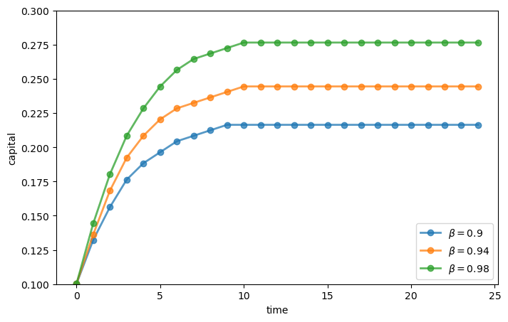
Finally, let us work on Exercise 2, where we plot the trajectories of the capital stock for three different discount factors, \(0.9\), \(0.94\), and \(0.98\), with initial condition \(k_0 = 0.1\).

discount_factors = (0.9, 0.94, 0.98)
k_init = 0.1

# Search for the index corresponding to k_init
k_init_ind = np.searchsorted(grid, k_init)

sample_size = 25

fig, ax = plt.subplots(figsize=(8,5))
ax.set_xlabel("time")
ax.set_ylabel("capital")
ax.set_ylim(0.10, 0.30)

# Create a new instance, not to modify the one used above
ddp0 = DiscreteDP(R, Q, β, s_indices, a_indices)

for beta in discount_factors:
    ddp0.beta = beta
    res0 = ddp0.solve()
    k_path_ind = res0.mc.simulate(init=k_init_ind, ts_length=sample_size)
    k_path = grid[k_path_ind]
    ax.plot(k_path, 'o-', lw=2, alpha=0.75, label=f'$\\beta = {beta}$')

ax.legend(loc='lower right')
plt.show()

_images/eb8882cc8b6fc46df77d7336ee033ddf5c941b02a1049ef3409320071d11f29f.png

4.7. Appendix: Algorithms #

This appendix covers the details of the solution algorithms implemented for DiscreteDP.

We will make use of the following notions of approximate optimality:

For \(\varepsilon > 0\), \(v\) is called an \(\varepsilon\)-approximation of \(v^*\) if \(\lVert v - v^*\rVert < \varepsilon\).
A policy \(\sigma \in \Sigma\) is called \(\varepsilon\)-optimal if \(v_{\sigma}\) is an \(\varepsilon\)-approximation of \(v^*\).

4.7.1. Value Iteration#

The DiscreteDP value iteration method implements value function iteration as follows

Choose any \(v^0 \in \mathbb{R}^n\), and specify \(\varepsilon > 0\); set \(i = 0\).
Compute \(v^{i+1} = T v^i\).
If \(\lVert v^{i+1} - v^i\rVert < [(1 - \beta) / (2\beta)] \varepsilon\), then go to step 4; otherwise, set \(i = i + 1\) and go to step 2.
Compute a \(v^{i+1}\)-greedy policy \(\sigma\), and return \(v^{i+1}\) and \(\sigma\).

Given \(\varepsilon > 0\), the value iteration algorithm

terminates in a finite number of iterations
returns an \(\varepsilon/2\)-approximation of the optimal value function and an \(\varepsilon\)-optimal policy function (unless iter_max is reached)

(While not explicit, in the actual implementation each algorithm is terminated if the number of iterations reaches iter_max)

4.7.2. Policy Iteration#

The DiscreteDP policy iteration method runs as follows

Choose any \(v^0 \in \mathbb{R}^n\) and compute a \(v^0\)-greedy policy \(\sigma^0\); set \(i = 0\).
Compute the value \(v_{\sigma^i}\) by solving the equation \(v = T_{\sigma^i} v\).
Compute a \(v_{\sigma^i}\)-greedy policy \(\sigma^{i+1}\); let \(\sigma^{i+1} = \sigma^i\) if possible.
If \(\sigma^{i+1} = \sigma^i\), then return \(v_{\sigma^i}\) and \(\sigma^{i+1}\); otherwise, set \(i = i + 1\) and go to step 2.

The policy iteration algorithm terminates in a finite number of iterations.

It returns an optimal value function and an optimal policy function (unless iter_max is reached).

4.7.3. Modified Policy Iteration#

The DiscreteDP modified policy iteration method runs as follows:

Choose any \(v^0 \in \mathbb{R}^n\), and specify \(\varepsilon > 0\) and \(k \geq 0\); set \(i = 0\).
Compute a \(v^i\)-greedy policy \(\sigma^{i+1}\); let \(\sigma^{i+1} = \sigma^i\) if possible (for \(i \geq 1\)).
Compute \(u = T v^i\) (\(= T_{\sigma^{i+1}} v^i\)). If \(\mathrm{span}(u - v^i) < [(1 - \beta) / \beta] \varepsilon\), then go to step 5; otherwise go to step 4.
- Span is defined by \(\mathrm{span}(z) = \max(z) - \min(z)\).
Compute \(v^{i+1} = (T_{\sigma^{i+1}})^k u\) (\(= (T_{\sigma^{i+1}})^{k+1} v^i\)); set \(i = i + 1\) and go to step 2.
Return \(v = u + [\beta / (1 - \beta)] [(\min(u - v^i) + \max(u - v^i)) / 2] \mathbf{1}\) and \(\sigma_{i+1}\).

Given \(\varepsilon > 0\), provided that \(v^0\) is such that \(T v^0 \geq v^0\), the modified policy iteration algorithm terminates in a finite number of iterations.

It returns an \(\varepsilon/2\)-approximation of the optimal value function and an \(\varepsilon\)-optimal policy function (unless iter_max is reached).

See also the documentation for DiscreteDP.