2. Continuous State Markov Chains#
In addition to what’s in Anaconda, this lecture will need the following libraries:
!pip install --upgrade quantecon
2.1. Overview#
In Finite Markov Chains, we learned about finite Markov chains, a relatively elementary class of stochastic dynamic models.
The present lecture extends this analysis to continuous (i.e., uncountable) state Markov chains.
Most stochastic dynamic models studied by economists either fit directly into this class or can be represented as continuous state Markov chains after minor modifications.
In this lecture, our focus will be on continuous Markov models that
evolve in discrete time
are often nonlinear
The fact that we accommodate nonlinear models here is significant, because linear stochastic models have their own highly developed toolset, as we’ll see later in Covariance Stationary Processes.
The question that interests us most is: Given a particular stochastic dynamic model, how will the state of the system evolve over time?
In particular,
What happens to the distribution of the state variables?
Is there anything we can say about the “average behavior” of these variables?
Is there a notion of “steady state” or “long-run equilibrium” that’s applicable to the model?
If so, how can we compute it?
Answering these questions will lead us to revisit many of the topics that occupied us in the finite state case, such as simulation, distribution dynamics, stability, ergodicity, etc.
Note
For some people, the term “Markov chain” always refers to a process with a finite or discrete state space. We follow the mainstream mathematical literature (e.g., [Meyn and Tweedie, 2009]) in using the term to refer to any discrete time Markov process.
Let’s begin with some imports:
import numpy as np
import matplotlib.pyplot as plt
from scipy.stats import lognorm, beta
from quantecon import LAE
from scipy.stats import norm, gaussian_kde
2.2. The density case#
You are probably aware that some distributions can be represented by densities and some cannot.
(For example, distributions on the real numbers \(\mathbb R\) that put positive probability on individual points have no density representation)
We are going to start our analysis by looking at Markov chains where the one-step transition probabilities have density representations.
The benefit is that the density case offers a very direct parallel to the finite case in terms of notation and intuition.
Once we’ve built some intuition we’ll cover the general case.
2.2.1. Definitions and basic properties#
In our lecture Finite Markov Chains, we studied discrete-time Markov chains that evolve on a finite state space \(S\).
In this setting, the dynamics of the model are described by a stochastic matrix — a nonnegative square matrix \(P = P[i, j]\) such that each row \(P[i, \cdot]\) sums to one.
The interpretation of \(P\) is that \(P[i, j]\) represents the probability of transitioning from state \(i\) to state \(j\) in one unit of time.
In symbols,
Equivalently,
\(P\) can be thought of as a family of distributions \(P[i, \cdot]\), one for each \(i \in S\)
\(P[i, \cdot]\) is the distribution of \(X_{t+1}\) given \(X_t = i\)
(As you probably recall, when using NumPy arrays, \(P[i, \cdot]\) is expressed as P[i,:])
In this section, we’ll allow \(S\) to be a subset of \(\mathbb R\), such as
\(\mathbb R\) itself
the positive reals \((0, \infty)\)
a bounded interval \((a, b)\)
The family of discrete distributions \(P[i, \cdot]\) will be replaced by a family of densities \(p(x, \cdot)\), one for each \(x \in S\).
Analogous to the finite state case, \(p(x, \cdot)\) is to be understood as the distribution (density) of \(X_{t+1}\) given \(X_t = x\).
More formally, a stochastic kernel on \(S\) is a function \(p \colon S \times S \to \mathbb R\) with the property that
\(p(x, y) \geq 0\) for all \(x, y \in S\)
\(\int p(x, y) dy = 1\) for all \(x \in S\)
(Integrals are over the whole space unless otherwise specified)
For example, let \(S = \mathbb R\) and consider the particular stochastic kernel \(p_w\) defined by
What kind of model does \(p_w\) represent?
The answer is, the (normally distributed) random walk
To see this, let’s find the stochastic kernel \(p\) corresponding to (2.2).
Recall that \(p(x, \cdot)\) represents the distribution of \(X_{t+1}\) given \(X_t = x\).
Letting \(X_t = x\) in (2.2) and considering the distribution of \(X_{t+1}\), we see that \(p(x, \cdot) = N(x, 1)\).
In other words, \(p\) is exactly \(p_w\), as defined in (2.1).
2.2.2. Connection to stochastic difference equations#
In the previous section, we made the connection between stochastic difference equation (2.2) and stochastic kernel (2.1).
In economics and time-series analysis we meet stochastic difference equations of all different shapes and sizes.
It will be useful for us if we have some systematic methods for converting stochastic difference equations into stochastic kernels.
To this end, consider the generic (scalar) stochastic difference equation given by
Here we assume that
\(\{ \xi_t \} \stackrel {\textrm{ IID }} {\sim} \phi\), where \(\phi\) is a given density on \(\mathbb R\)
\(\mu\) and \(\sigma\) are given functions on \(S\), with \(\sigma(x) > 0\) for all \(x\)
Example 1: The random walk (2.2) is a special case of (2.3), with \(\mu(x) = x\) and \(\sigma(x) = 1\).
Example 2: Consider the ARCH model
Alternatively, we can write the model as
This is a special case of (2.3) with \(\mu(x) = \alpha x\) and \(\sigma(x) = (\beta + \gamma x^2)^{1/2}\).
Example 3: With stochastic production and a constant savings rate, the one-sector neoclassical growth model leads to a law of motion for capital per worker such as
Here
\(s\) is the rate of savings
\(A_{t+1}\) is a production shock
The \(t+1\) subscript indicates that \(A_{t+1}\) is not visible at time \(t\)
\(\delta\) is a depreciation rate
\(f \colon \mathbb R_+ \to \mathbb R_+\) is a production function satisfying \(f(k) > 0\) whenever \(k > 0\)
(The fixed savings rate can be rationalized as the optimal policy for a particular set of technologies and preferences (see [Ljungqvist and Sargent, 2018], section 3.1.2), although we omit the details here).
Equation (2.5) is a special case of (2.3) with \(\mu(x) = (1 - \delta)x\) and \(\sigma(x) = s f(x)\).
Now let’s obtain the stochastic kernel corresponding to the generic model (2.3).
To find it, note first that if \(U\) is a random variable with density \(f_U\), and \(V = a + b U\) for some constants \(a,b\) with \(b > 0\), then the density of \(V\) is given by
(The proof is below. For a multidimensional version see EDTC, theorem 8.1.3).
Taking (2.6) as given for the moment, we can obtain the stochastic kernel \(p\) for (2.3) by recalling that \(p(x, \cdot)\) is the conditional density of \(X_{t+1}\) given \(X_t = x\).
In the present case, this is equivalent to stating that \(p(x, \cdot)\) is the density of \(Y := \mu(x) + \sigma(x) \, \xi_{t+1}\) when \(\xi_{t+1} \sim \phi\).
Hence, by (2.6),
For example, the growth model in (2.5) has stochastic kernel
where \(\phi\) is the density of \(A_{t+1}\).
(Regarding the state space \(S\) for this model, a natural choice is \((0, \infty)\) — in which case \(\sigma(x) = s f(x)\) is strictly positive for all \(x\) as required)
2.2.3. Distribution dynamics#
In this section of our lecture on finite Markov chains, we asked the following question: If
\(\{X_t\}\) is a Markov chain with stochastic matrix \(P\)
the distribution of \(X_t\) is known to be \(\psi_t\)
then what is the distribution of \(X_{t+1}\)?
Letting \(\psi_{t+1}\) denote the distribution of \(X_{t+1}\), the answer we gave was that
This intuitive equality states that the probability of being at \(j\) tomorrow is the probability of visiting \(i\) today and then going on to \(j\), summed over all possible \(i\).
In the density case, we just replace the sum with an integral and probability mass functions with densities, yielding
It is convenient to think of this updating process in terms of an operator.
(An operator is just a function, but the term is usually reserved for a function that sends functions into functions)
Let \(\mathscr D\) be the set of all densities on \(S\), and let \(P\) be the operator from \(\mathscr D\) to itself that takes density \(\psi\) and sends it into new density \(\psi P\), where the latter is defined by
This operator is usually called the Markov operator corresponding to \(p\).
Note
Unlike most operators, we write \(P\) to the right of its argument, instead of to the left (i.e., \(\psi P\) instead of \(P \psi\)). This is a common convention, with the intention being to maintain the parallel with the finite case — see here
With this notation, we can write (2.9) more succinctly as \(\psi_{t+1}(y) = (\psi_t P)(y)\) for all \(y\), or, dropping the \(y\) and letting “\(=\)” indicate equality of functions,
Equation (2.11) tells us that if we specify a distribution for \(\psi_0\), then the entire sequence of future distributions can be obtained by iterating with \(P\).
It’s interesting to note that (2.11) is a deterministic difference equation.
Thus, by converting a stochastic difference equation such as (2.3) into a stochastic kernel \(p\) and hence an operator \(P\), we convert a stochastic difference equation into a deterministic one (albeit in a much higher dimensional space).
Note
Some people might be aware that discrete Markov chains are in fact a special case of the continuous Markov chains we have just described. The reason is that probability mass functions are densities with respect to the counting measure.
2.2.4. Computation#
To learn about the dynamics of a given process, it’s useful to compute and study the sequences of densities generated by the model.
One way to do this is to try to implement the iteration described by (2.10) and (2.11) using numerical integration.
However, to produce \(\psi P\) from \(\psi\) via (2.10), you would need to integrate at every \(y\), and there is a continuum of such \(y\).
Another possibility is to discretize the model, but this introduces errors of unknown size.
A nicer alternative in the present setting is to combine simulation with an elegant estimator called the look-ahead estimator.
Let’s go over the ideas with reference to the growth model discussed above, the dynamics of which we repeat here for convenience:
Our aim is to compute the sequence \(\{ \psi_t \}\) associated with this model and fixed initial condition \(\psi_0\).
To approximate \(\psi_t\) by simulation, recall that, by definition, \(\psi_t\) is the density of \(k_t\) given \(k_0 \sim \psi_0\).
If we wish to generate observations of this random variable, all we need to do is
draw \(k_0\) from the specified initial condition \(\psi_0\)
draw the shocks \(A_1, \ldots, A_t\) from their specified density \(\phi\)
compute \(k_t\) iteratively via (2.12)
If we repeat this \(n\) times, we get \(n\) independent observations \(k_t^1, \ldots, k_t^n\).
With these draws in hand, the next step is to generate some kind of representation of their distribution \(\psi_t\).
A naive approach would be to use a histogram, or perhaps a smoothed histogram using SciPy’s gaussian_kde function.
However, in the present setting, there is a much better way to do this, based on the look-ahead estimator.
With this estimator, to construct an estimate of \(\psi_t\), we actually generate \(n\) observations of \(k_{t-1}\), rather than \(k_t\).
Now we take these \(n\) observations \(k_{t-1}^1, \ldots, k_{t-1}^n\) and form the estimate
where \(p\) is the growth model stochastic kernel in (2.8).
What is the justification for this slightly surprising estimator?
The idea is that, by the strong law of large numbers,
with probability one as \(n \to \infty\).
Here the first equality is by the definition of \(\psi_{t-1}\), and the second is by (2.9).
We have just shown that our estimator \(\psi_t^n(y)\) in (2.13) converges almost surely to \(\psi_t(y)\), which is just what we want to compute.
In fact, much stronger convergence results are true (see, for example, this paper).
2.2.5. Implementation#
A class called LAE for estimating densities by this technique can be found in lae.py.
Given our use of the __call__ method, an instance of LAE acts as a callable object, which is essentially a function that can store its own data (see this discussion).
This function returns the right-hand side of (2.13) using
the data and stochastic kernel that it stores as its instance data
the value \(y\) as its argument
The function is vectorized, in the sense that if psi is such an instance and y is an array, then the call psi(y) acts elementwise.
(This is the reason that we reshaped X and y inside the class — to make vectorization work)
Because the implementation is fully vectorized, it is about as efficient as it would be in C or Fortran.
2.2.6. Example#
The following code is an example of usage for the stochastic growth model described above
# == Define parameters == #
s = 0.2
δ = 0.1
a_σ = 0.4                    # A = exp(B) where B ~ N(0, a_σ**2)
α = 0.4                      # We set f(k) = k**α
ψ_0 = beta(5, 5, scale=0.5)  # Initial distribution
ϕ = lognorm(a_σ)
rng = np.random.default_rng(1234)


def p(x, y):
    """
    Stochastic kernel for the growth model with Cobb-Douglas production.
    Both x and y must be strictly positive.
    """
    d = s * x**α
    return ϕ.pdf((y - (1 - δ) * x) / d) / d

n = 10000    # Number of observations at each date t
T = 30       # Compute density of k_t at 1,...,T

# == Generate matrix s.t. t-th column is n observations of k_t == #
k = np.empty((n, T))
A = ϕ.rvs((n, T), random_state=rng)
k[:, 0] = ψ_0.rvs(n, random_state=rng)  # Draw first column from initial distribution
for t in range(T-1):
    k[:, t+1] = s * A[:, t] * k[:, t]**α + (1 - δ) * k[:, t]

# == Generate T instances of LAE using this data, one for each date t == #
laes = [LAE(p, k[:, t]) for t in range(T)]

# == Plot == #
fig, ax = plt.subplots()
ygrid = np.linspace(0.01, 4.0, 200)
greys = [str(g) for g in np.linspace(0.0, 0.8, T)]
greys.reverse()
for ψ, g in zip(laes, greys):
    ax.plot(ygrid, ψ(ygrid), color=g, lw=2, alpha=0.6)
ax.set_xlabel('capital')
plt.show()
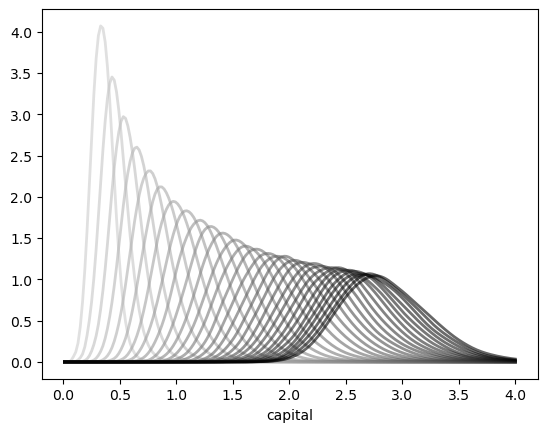
Fig. 2.1 Density of \(k_1\) (lighter) to \(k_T\) (darker)#
The figure shows part of the density sequence \(\{\psi_t\}\), with each density computed via the look-ahead estimator.
Notice that the sequence of densities shown in the figure seems to be converging — more on this in just a moment.
Another quick comment is that each of these distributions could be interpreted as a cross-sectional distribution (recall this discussion).
2.3. Beyond densities#
Up until now, we have focused exclusively on continuous state Markov chains where all conditional distributions \(p(x, \cdot)\) are densities.
As discussed above, not all distributions can be represented as densities.
If the conditional distribution of \(X_{t+1}\) given \(X_t = x\) cannot be represented as a density for some \(x \in S\), then we need a slightly different theory.
The ultimate option is to switch from densities to probability measures, but not all readers will be familiar with measure theory.
We can, however, construct a fairly general theory using distribution functions.
2.3.1. Example and definitions#
To illustrate the issues, recall that Hopenhayn and Rogerson [1993] study a model of firm dynamics where individual firm productivity follows the exogenous process
As is, this fits into the density case we treated above.
However, the authors wanted this process to take values in \([0, 1]\), so they added boundaries at the endpoints 0 and 1.
One way to write this is
If you think about it, you will see that for any given \(x \in [0, 1]\), the conditional distribution of \(X_{t+1}\) given \(X_t = x\) puts positive probability mass on 0 and 1.
Hence it cannot be represented as a density.
What we can do instead is use cumulative distribution functions (CDFs).
To this end, set
This family of CDFs \(G(x, \cdot)\) plays a role analogous to the stochastic kernel in the density case.
The distribution dynamics in (2.9) are then replaced by
Here \(F_t\) and \(F_{t+1}\) are CDFs representing the distribution of the current state and next period state.
The intuition behind (2.14) is essentially the same as for (2.9).
2.3.2. Computation#
If you wish to compute these CDFs, you cannot use the look-ahead estimator as before.
Indeed, you should not use any density estimator, since the objects you are estimating/computing are not densities.
One good option is simulation as before, combined with the empirical distribution function.
2.4. Stability#
In our lecture Finite Markov Chains, we also studied stationarity, stability and ergodicity.
Here we will cover the same topics for the continuous case.
We will, however, treat only the density case (as in this section), where the stochastic kernel is a family of densities.
The general case is relatively similar — references are given below.
2.4.1. Theoretical results#
Analogous to the finite case, given a stochastic kernel \(p\) and corresponding Markov operator as defined in (2.10), a density \(\psi^*\) on \(S\) is called stationary for \(P\) if it is a fixed point of the operator \(P\).
In other words,
As with the finite case, if \(\psi^*\) is stationary for \(P\), and the distribution of \(X_0\) is \(\psi^*\), then, in view of (2.11), \(X_t\) will have this same distribution for all \(t\).
Hence \(\psi^*\) is the stochastic equivalent of a steady state.
In the finite case, we learned that at least one stationary distribution exists, although there may be many.
When the state space is infinite, the situation is more complicated.
Even existence can fail very easily.
For example, the random walk model has no stationary density (see, e.g., EDTC, p. 210).
However, there are well-known conditions under which a stationary density \(\psi^*\) exists.
With additional conditions, we can also get a unique stationary density (\(\psi \in \mathscr D \text{ and } \psi = \psi P \implies \psi = \psi^*\)), and also global convergence in the sense that
This combination of existence, uniqueness and global convergence in the sense of (2.16) is often referred to as global stability.
Under very similar conditions, we get ergodicity, which means that
for any (measurable) function \(h \colon S \to \mathbb R\) such that the right-hand side is finite.
Note that the convergence in (2.17) does not depend on the distribution (or value) of \(X_0\).
This is actually very important for simulation — it means we can learn about \(\psi^*\) (i.e., approximate the right-hand side of (2.17) via the left-hand side) without requiring any special knowledge about what to do with \(X_0\).
So what are these conditions we require to get global stability and ergodicity?
In essence, it must be the case that
Probability mass does not drift off to the “edges” of the state space.
Sufficient “mixing” obtains.
For one such set of conditions see theorem 8.2.14 of EDTC.
In addition
[Stokey et al., 1989] contains a classic (but slightly outdated) treatment of these topics.
From the mathematical literature, [Lasota and MacKey, 1994] and [Meyn and Tweedie, 2009] give outstanding in-depth treatments.
Section 8.1.2 of EDTC provides detailed intuition, and section 8.3 gives additional references.
EDTC, section 11.3.4 provides a specific treatment for the growth model we considered in this lecture.
2.4.2. An example of stability#
As stated above, the growth model treated here is stable under mild conditions on the primitives.
See EDTC, section 11.3.4 for more details.
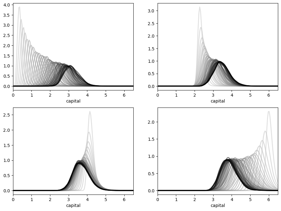
We can see this stability in action — in particular, the convergence in (2.16) — by simulating the path of densities from various initial conditions.
Here is such a figure.
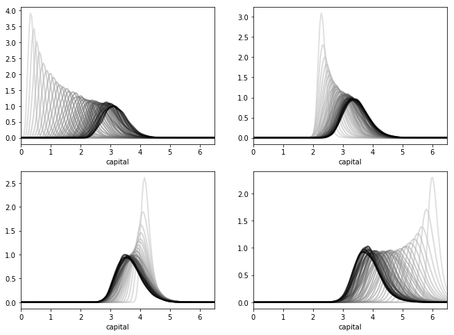
Fig. 2.2 Density sequences from four different initial conditions#
All sequences are converging towards the same limit, regardless of their initial condition.
The details regarding initial conditions and so on are given in this exercise, where you are asked to replicate the figure.
2.4.3. Computing stationary densities#
In the preceding figure, each sequence of densities is converging towards the unique stationary density \(\psi^*\).
Even from this figure, we can get a fair idea what \(\psi^*\) looks like, and where its mass is located.
However, there is a much more direct way to estimate the stationary density, and it involves only a slight modification of the look-ahead estimator.
Let’s say that we have a model of the form (2.3) that is stable and ergodic.
Let \(p\) be the corresponding stochastic kernel, as given in (2.7).
To approximate the stationary density \(\psi^*\), we can simply generate a long time-series \(X_0, X_1, \ldots, X_n\) and estimate \(\psi^*\) via
This is essentially the same as the look-ahead estimator (2.13), except that now the observations we generate are a single time-series, rather than a cross-section.
The justification for (2.18) is that, with probability one as \(n \to \infty\),
where the convergence is by (2.17) and the equality on the right is by (2.15).
The right-hand side is exactly what we want to compute.
On top of this asymptotic result, it turns out that the rate of convergence for the look-ahead estimator is very good.
The first exercise helps illustrate this point.
2.5. Exercises#
Exercise 2.1
Consider the simple threshold autoregressive model
This is one of those rare nonlinear stochastic models where an analytical expression for the stationary density is available.
In particular, provided that \(|\theta| < 1\), there is a unique stationary density \(\psi^*\) given by
Here \(\phi\) is the standard normal density and \(\Phi\) is the standard normal cdf.
As an exercise, compute the look-ahead estimate of \(\psi^*\), as defined in (2.18), and compare it with \(\psi^*\) in (2.20) to see whether they are indeed close for large \(n\).
In doing so, set \(\theta = 0.8\) and \(n = 500\).
The next figure shows the result of such a computation
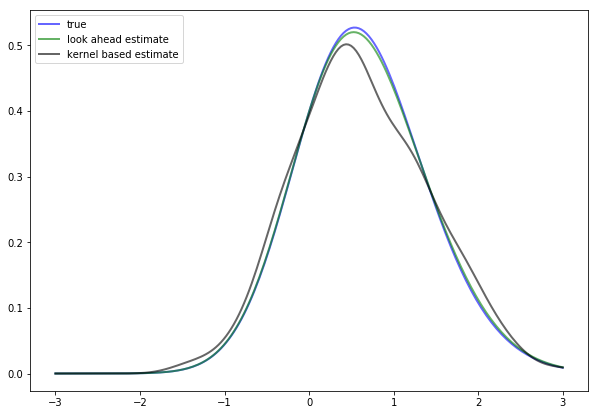
The additional density (black line) is a nonparametric kernel density estimate, added to the solution for illustration.
(You can try to replicate it before looking at the solution if you want to)
As you can see, the look-ahead estimator is a much tighter fit than the kernel density estimator.
If you repeat the simulation you will see that this is consistently the case.
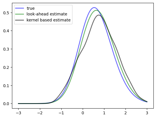
Solution
Look-ahead estimation of a TAR stationary density, where the TAR model is
and \(\xi_t \sim N(0,1)\).
Try running at n = 10, 100, 1000, 10000 to get an idea of the speed of convergence
ϕ = norm()
n = 500
θ = 0.8
rng = np.random.default_rng(1234)
# == Frequently used constants == #
d = np.sqrt(1 - θ**2)
δ = θ / d

def ψ_star(y):
    "True stationary density of the TAR Model"
    return 2 * norm.pdf(y) * norm.cdf(δ * y)

def p(x, y):
    "Stochastic kernel for the TAR model."
    return ϕ.pdf((y - θ * np.abs(x)) / d) / d

Z = ϕ.rvs(n, random_state=rng)
X = np.empty(n)
X[0] = 0
for t in range(n-1):
    X[t+1] = θ * np.abs(X[t]) + d * Z[t]
ψ_est = LAE(p, X)
k_est = gaussian_kde(X)

fig, ax = plt.subplots()
ys = np.linspace(-3, 3, 200)
ax.plot(ys, ψ_star(ys), 'b-', lw=2, alpha=0.6, label='true')
ax.plot(ys, ψ_est(ys), 'g-', lw=2, alpha=0.6, label='look-ahead estimate')
ax.plot(ys, k_est(ys), 'k-', lw=2, alpha=0.6, label='kernel based estimate')
ax.legend(loc='upper left')
plt.show()
Exercise 2.2
Replicate the figure on global convergence shown above.
The densities come from the stochastic growth model treated at the start of the lecture.
Begin with the code found above.
Use the same parameters.
For the four initial distributions, use the shifted beta distributions
ψ_0 = beta(5, 5, scale=0.5, loc=i*2)
Solution
Here’s one program that does the job
# == Define parameters == #
s = 0.2
δ = 0.1
a_σ = 0.4                                # A = exp(B) where B ~ N(0, a_σ**2)
α = 0.4                                  # f(k) = k**α

ϕ = lognorm(a_σ)
rng = np.random.default_rng(1234)

def p(x, y):
    "Stochastic kernel, vectorized in x.  Both x and y must be positive."
    d = s * x**α
    return ϕ.pdf((y - (1 - δ) * x) / d) / d

n = 1000                            # Number of observations at each date t
T = 40                              # Compute density of k_t at 1,...,T

fig, axes = plt.subplots(2, 2, figsize=(11, 8))
axes = axes.flatten()
xmax = 6.5

for i in range(4):
    ax = axes[i]
    ax.set_xlim(0, xmax)
    ψ_0 = beta(5, 5, scale=0.5, loc=i*2)  # Initial distribution

    # == Generate matrix s.t. t-th column is n observations of k_t == #
    k = np.empty((n, T))
    A = ϕ.rvs((n, T), random_state=rng)
    k[:, 0] = ψ_0.rvs(n, random_state=rng)
    for t in range(T-1):
        k[:, t+1] = s * A[:,t] * k[:, t]**α + (1 - δ) * k[:, t]

    # == Generate T instances of lae using this data, one for each t == #
    laes = [LAE(p, k[:, t]) for t in range(T)]

    ygrid = np.linspace(0.01, xmax, 150)
    greys = [str(g) for g in np.linspace(0.0, 0.8, T)]
    greys.reverse()
    for ψ, g in zip(laes, greys):
        ax.plot(ygrid, ψ(ygrid), color=g, lw=2, alpha=0.6)
    ax.set_xlabel('capital')
plt.show()
Exercise 2.3
A common way to compare distributions visually is with boxplots.
To illustrate, let’s generate three artificial data sets and compare them with a boxplot.
The three data sets we will use are:
Here is the code and figure:
n = 500
rng = np.random.default_rng(1234)
x = rng.standard_normal(n)        # N(0, 1)
x = np.exp(x)                     # Map x to lognormal
y = rng.standard_normal(n) + 2.0  # N(2, 1)
z = rng.standard_normal(n) + 4.0  # N(4, 1)

fig, ax = plt.subplots()
ax.boxplot([x, y, z])
ax.set_xticks((1, 2, 3))
ax.set_ylim(-2, 14)
ax.set_xticklabels(('$X$', '$Y$', '$Z$'), fontsize=16)
plt.show()
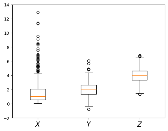
Each data set is represented by a box, where the top and bottom of the box are the third and first quartiles of the data, and the red line in the center is the median.
The boxes give some indication as to
the location of probability mass for each sample
whether the distribution is right-skewed (as is the lognormal distribution), etc
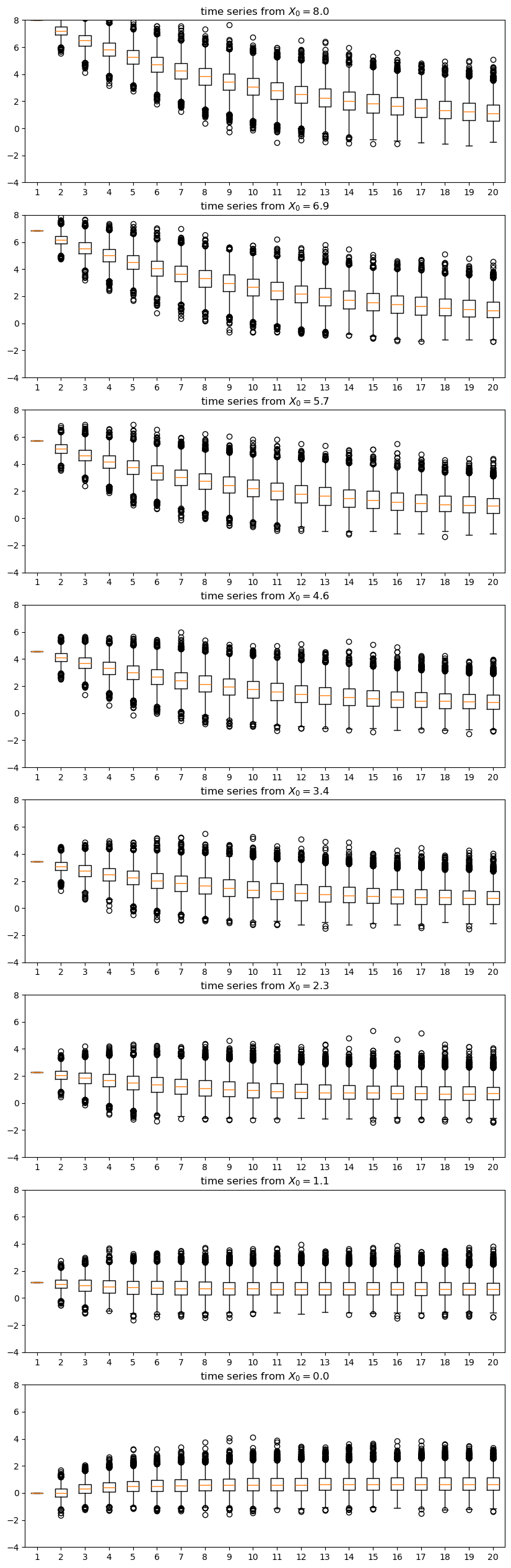
Now let’s put these ideas to use in a simulation.
Consider the threshold autoregressive model in (2.19).
We know that the distribution of \(X_t\) will converge to (2.20) whenever \(|\theta| < 1\).
Let’s observe this convergence from different initial conditions using boxplots.
In particular, the exercise is to generate J boxplot figures, one for each initial condition \(X_0\) in
initial_conditions = np.linspace(8, 0, J)
For each \(X_0\) in this set,
Generate \(k\) time-series of length \(n\), each starting at \(X_0\) and obeying (2.19).
Create a boxplot representing \(n\) distributions, where the \(t\)-th distribution shows the \(k\) observations of \(X_t\).
Use \(\theta = 0.9, n = 20, k = 5000, J = 8\)
Solution
Here’s a possible solution.
Note the way we use vectorized code to simulate the \(k\) time series for one boxplot all at once
n = 20
k = 5000
J = 8

θ = 0.9
d = np.sqrt(1 - θ**2)
δ = θ / d
rng = np.random.default_rng(1234)

fig, axes = plt.subplots(J, 1, figsize=(10, 4*J))
initial_conditions = np.linspace(8, 0, J)
X = np.empty((k, n))

for j in range(J):

    axes[j].set_ylim(-4, 8)
    axes[j].set_title(f'time series from $X_0 = {initial_conditions[j]:.1f}$')

    Z = rng.standard_normal((k, n))
    X[:, 0] = initial_conditions[j]
    for t in range(1, n):
        X[:, t] = θ * np.abs(X[:, t-1]) + d * Z[:, t]
    axes[j].boxplot(X)

plt.show()
2.6. Appendix#
Here’s the proof of (2.6).
Let \(F_U\) and \(F_V\) be the cumulative distributions of \(U\) and \(V\) respectively.
By the definition of \(V\), we have \(F_V(v) = \mathbb P \{ a + b U \leq v \} = \mathbb P \{ U \leq (v - a) / b \}\).
In other words, \(F_V(v) = F_U ( (v - a)/b )\).
Differentiating with respect to \(v\) yields (2.6).