43. Time Inconsistency of Ramsey Plans#

In addition to what’s in Anaconda, this lecture will need the following libraries:

!pip install --upgrade quantecon

43.1. Overview#

This lecture describes a linear-quadratic version of a model that Guillermo Calvo [Calvo, 1978] used to analyze the time inconsistency of optimal government plans.

We use the model as a laboratory in which we explore consequences of different timing protocols for government decision making.

The model focuses on intertemporal tradeoffs between

benefits that anticipations of future deflation generate by decreasing costs of holding real money balances and thereby increasing a representative agent’s liquidity, as measured by his or her holdings of real money balances, and
costs associated with the distorting taxes that the government must levy in order to acquire the paper money that it will destroy in order to generate anticipated deflation

Model features include

rational expectations
alternative possible timing protocols for government choices of a sequence of money growth rates
costly government actions at all dates $t \geq 1$ that increase household utilities at dates before $t$
alternative possible sets of Bellman equations, one set for each timing protocol
- for example, in a timing protocol used to pose a Ramsey plan, a government chooses an infinite sequence of money supply growth rates once and for all at time $0$.
- in this timing protocol, there are two value functions and associated Bellman equations, one that expresses a representative private expectation of future inflation as a function of current and future government actions, another that describes the value function of a Ramsey planner
- in other timing protocols, other Bellman equations and associated value functions will appear

A theme of this lecture is that timing protocols for government decisions affect outcomes.

We’ll use ideas from papers by Cagan [Cagan, 1956], Calvo [Calvo, 1978], and Chang [Chang, 1998] as well as from chapter 19 of [Ljungqvist and Sargent, 2018].

In addition, we’ll use ideas from linear-quadratic dynamic programming described in Linear Quadratic Control as applied to Ramsey problems in Stackelberg plans.

We specify model fundamentals in ways that allow us to use linear-quadratic discounted dynamic programming to compute an optimal government plan under each of our timing protocols.

A sister lecture Machine Learning a Ramsey Plan studies some of the same models but does not use dynamic programming.

Instead it uses a machine learning approach that does not explicitly recognize the recursive structure structure of the Ramsey problem that Chang [Chang, 1998] saw and that we exploit in this lecture.

In addition to what’s in Anaconda, this lecture will use the following libraries:

!pip install --upgrade quantecon

We’ll start with some imports:

import numpy as np
from quantecon import LQ
import matplotlib.pyplot as plt
from matplotlib.ticker import FormatStrFormatter
import pandas as pd
from IPython.display import display, Math

43.2. Model Components#

There is no uncertainty.

Let:

$p_t$ be the log of the price level
$m_t$ be the log of nominal money balances
$\theta_t = p_{t+1} - p_t$ be the net rate of inflation between $t$ and $t+1$
$\mu_t = m_{t+1} - m_t$ be the net rate of growth of nominal balances

The demand for real balances is governed by a discrete time version of Sargent and Wallace’s [Sargent and Wallace, 1973] perfect foresight version of a Cagan [Cagan, 1956] demand function for real balances:

(43.1)#\[m_t - p_t = -\alpha(p_{t+1} - p_t) \: , \: \alpha > 0\]

for $t \geq 0$.

Equation (43.1) asserts that the demand for real balances is inversely related to the public’s expected rate of inflation, which equals the actual rate of inflation because there is no uncertainty here.

Note

When there is no uncertainty, an assumption of rational expectations becomes equivalent to perfect foresight. [Sargent, 1977] presents a rational expectations version of the model when there is uncertainty.

Subtracting the demand function (43.1) at time $t$ from the time $t+1$ version of this demand function gives

\[ \mu_t - \theta_t = -\alpha \theta_{t+1} + \alpha \theta_t \]

(43.2)#\[\theta_t = \frac{\alpha}{1+\alpha} \theta_{t+1} + \frac{1}{1+\alpha} \mu_t\]

Because $\alpha > 0$, $0 < \frac{\alpha}{1+\alpha} < 1$.

Definition: For scalar $b_t$, let $L^2$ be the space of sequences $\{b_t\}_{t=0}^\infty$ satisfying

\[ \sum_{t=0}^\infty b_t^2 < +\infty \]

We say that a sequence that belongs to $L^2$ is square summable.

When we assume that the sequence $\vec \mu = \{\mu_t\}_{t=0}^\infty$ is square summable and we require that the sequence $\vec \theta = \{\theta_t\}_{t=0}^\infty$ is square summable, the linear difference equation (43.2) can be solved forward to get:

(43.3)#\[\theta_t = \frac{1}{1+\alpha} \sum_{j=0}^\infty \left(\frac{\alpha}{1+\alpha}\right)^j \mu_{t+j}\]

Insight: Chang [Chang, 1998] noted that equations (43.1) and (43.3) show that $\theta_t$ intermediates how choices of $\mu_{t+j}, \ j=0, 1, \ldots$ impinge on time $t$ real balances $m_t - p_t = -\alpha \theta_t$.

An equivalence class of continuation money growth sequences $\{\mu_{t+j}\}_{j=0}^\infty$ deliver the same $\theta_t$.

We shall use this insight to simplify our analysis of alternative government policy problems.

That future rates of money creation influence earlier rates of inflation makes timing protocols matter for modeling optimal government policies.

We can represent restriction (43.3) as

(43.4)#\[\begin{split} \begin{bmatrix} 1 \\ \theta_{t+1} \end{bmatrix} = \begin{bmatrix} 1 & 0 \\ 0 & \frac{1+\alpha}{\alpha} \end{bmatrix} \begin{bmatrix} 1 \\ \theta_{t} \end{bmatrix} + \begin{bmatrix} 0 \\ -\frac{1}{\alpha} \end{bmatrix} \mu_t \end{split}\]

(43.5)#\[x_{t+1} = A x_t + B \mu_t\]

Even though $\theta_0$ is to be determined by our model and so is not an initial condition, as it ordinarily would be in the state-space model described in our lecture on Linear Quadratic Control, we nevertheless write the model in the state-space form (43.5).

We use form (43.5) because we want to apply an approach described in our lecture on Stackelberg plans.

Notice that $\frac{1+\alpha}{\alpha} > 1$ is an eigenvalue of transition matrix $A$ that threatens to destabilize the state-space system.

Indeed, for arbitrary, $\vec \mu = \{\mu_t\}_{t=0}^\infty$ sequences, $\vec \theta = \{\theta_t\}_{t=0}^\infty$ will not be square summable.

But the government planner will design a decision rule for $\mu_t$ that stabilizes the system and renders $\vec \theta$ square summable.

The government values a representative household’s utility of real balances at time $t$ according to the utility function

(43.6)#\[U(m_t - p_t) = u_0 + u_1 (m_t - p_t) - \frac{u_2}{2} (m_t - p_t)^2, \quad u_0 > 0, u_1 > 0, u_2 > 0\]

The money demand function (43.1) and the utility function (43.6) imply that

(43.7)#\[ U(-\alpha \theta_t) = u_0 + u_1 (-\alpha \theta_t) -\frac{u_2}{2}(-\alpha \theta_t)^2 . \]

43.3. Friedman’s Optimal Rate of Deflation#

According to (43.7), the bliss level of real balances is $\frac{u_1}{u_2}$ and the inflation rate that attains it is

(43.8)#\[ \theta_t = \theta^* = -\frac{u_1}{u_2 \alpha} \]

Milton Friedman recommended that the government withdraw and destroy money at a rate that implies an inflation rate given by (43.8).

In our setting, that could be accomplished by setting

(43.9)#\[ \mu_t = \mu^* = \theta^* , t \geq 0 \]

where $\theta^*$ is given by equation (43.8).

Milton Friedman assumed that the taxes that government imposes to collect money at rate $\mu_t$ do not distort economic decisions, e.g., they are lump-sum taxes.

43.4. Calvo’s Distortion#

The starting point of Calvo [Calvo, 1978] and Chang [Chang, 1998] is that lump sum taxes are not available.

Instead, the government acquires money by levying taxes that distort decisions and thereby impose costs on the representative consumer.

In the models of Calvo [Calvo, 1978] and Chang [Chang, 1998], the government takes those tax-distortion costs into account.

The government balances the costs of imposing the distorting taxes needed to acquire the money that it destroys in order to generate deflation against the benefits that expected deflation generates by raising the representative household’s real money balances.

Let’s see how the government does that.

Via equation (43.3), a government plan $\vec \mu = \{\mu_t \}_{t=0}^\infty$ leads to a sequence of inflation outcomes $\vec \theta = \{ \theta_t \}_{t=0}^\infty$.

The government incurs social costs $\frac{c}{2} \mu_t^2$ at $t$ when it changes the stock of nominal money balances at rate $\mu_t$.

Therefore, the one-period welfare function of a benevolent government is:

(43.10)#\[\begin{split}s(\theta_t, \mu_t) := - r(x_t,\mu_t) = \begin{bmatrix} 1 \\ \theta_t \end{bmatrix}' \begin{bmatrix} u_0 & -\frac{u_1 \alpha}{2} \\ -\frac{u_1 \alpha}{2} & -\frac{u_2 \alpha^2}{2} \end{bmatrix} \begin{bmatrix} 1 \\ \theta_t \end{bmatrix} - \frac{c}{2} \mu_t^2 = - x_t'Rx_t - Q \mu_t^2\end{split}\]

The government’s time $0$ value is

(43.11)#\[v_0 = - \sum_{t=0}^\infty \beta^t r(x_t,\mu_t) = \sum_{t=0}^\infty \beta^t s(\theta_t,\mu_t)\]

where $\beta \in (0,1)$ is a discount factor.

Note

We define $ r(x_t,\mu_t) := - s(\theta_t, \mu_t) $ in order to represent the government’s maximization problem in terms of our Python code for solving linear quadratic discounted dynamic programs. In first LQ control lecture and some other quantecon lectures, we formulated these as loss minimization problems.

The government’s time $t$ continuation value $v_t$ is

(43.12)#\[ v_t = \sum_{j=0}^\infty \beta^j s(\theta_{t+j}, \mu_{t+j}) . \]

We can represent dependence of $v_0$ on $(\vec \theta, \vec \mu)$ recursively via the difference equation

(43.13)#\[v_t = s(\theta_t, \mu_t) + \beta v_{t+1}\]

It is useful to evaluate (43.13) under a time-invariant money growth rate $\mu_t = \bar \mu$ that according to equation (43.3) would bring forth a constant inflation rate equal to $\bar \mu$.

Under that policy,

(43.14)#\[ v_t = V(\bar \mu) = \frac{s(\bar \mu, \bar \mu)}{1-\beta} \]

for all $t \geq 0$.

Values of $V(\bar \mu)$ computed according to formula (43.14) for three different values of $\bar \mu$ will play important roles below.

$V(\mu^{MPE})$ is the value of attained by the government in a Markov perfect equilibrium
$V(\mu^R_\infty)$ is the value that a continuation Ramsey planner attains at $t \rightarrow +\infty$
- We shall discover that $V(\mu^R_\infty)$ is the worst continuation value attained along a Ramsey plan
$V(\mu^{CR})$ is the value of attained by the government in a constrained to constant $\mu$ equilibrium

43.5. Structure#

The following structure is induced by a representative agent’s behavior as summarized by the demand function for money (43.1) that leads to equation (43.3), which tells how future settings of $\mu$ affect the current value of $\theta$.

Equation (43.3) maps a policy sequence of money growth rates $\vec \mu =\{\mu_t\}_{t=0}^\infty \in L^2$ into an inflation sequence $\vec \theta = \{\theta_t\}_{t=0}^\infty \in L^2$.

These in turn induce a discounted value to a government sequence $\vec v = \{v_t\}_{t=0}^\infty \in L^2$ that satisfies recursion (43.13).

Thus, a triple of sequences $(\vec \mu, \vec \theta, \vec v)$ depends on a sequence $\vec \mu \in L^2$.

At this point $\vec \mu \in L^2$ is an arbitrary exogenous policy.

A theory of government decisions will make $\vec \mu$ endogenous, i.e., a theoretical output instead of an input.

43.5.1. Intertemporal Aspects#

Criterion function (43.11) and the constraint system (43.5) exhibit the following structure:

Setting the money growth rate $\mu_t \neq 0$ imposes costs $\frac{c}{2} \mu_t^2$ at time $t$ and at no other times; but
The money growth rate $\mu_t$ affects the government’s one-period utilities at all dates $s = 0, 1, \ldots, t$.

This structure sets the stage for the emergence of a time-inconsistent optimal government plan under a Ramsey timing protocol

it is also called a Stackelberg timing protocol.

We’ll study outcomes under a Ramsey timing protocol.

We’ll also study outcomes under other timing protocols.

43.6. Three Timing Protocols#

We consider three models of government policy making that differ in

what a policymaker chooses, either a sequence $\vec \mu$ or just $\mu_t$ in a single period $t$.
when a policymaker chooses, either once and for all at time $0$, or at one or more times $t \geq 0$.
what a policymaker assumes about how its choice of $\mu_t$ affects the representative agent’s expectations about earlier and later inflation rates.

In two of our models, a single policymaker chooses a sequence $\{\mu_t\}_{t=0}^\infty$ once and for all, knowing how $\mu_t$ affects household one-period utilities at dates $s = 0, 1, \ldots, t-1$

these two models thus employ a Ramsey or Stackelberg timing protocol.

In a third model, there is a sequence of policymaker indexed by $t \in \{0, 1, \ldots\}$, each of whom sets only $\mu_t$.

a time $t$ policymaker cares only about $v_t$ and ignores effects that its choice of $\mu_t$ has on $v_s$ at dates $s = 0, 1, \ldots, t-1$.

The three models differ with respect to timing protocols, constraints on government choices, and government policymakers’ beliefs about how their decisions affect the representative agent’s beliefs about future government decisions.

The models are distinguished by their having either

A single Ramsey planner that chooses a sequence $\{\mu_t\}_{t=0}^\infty$ once and for all at time $0$; or
A single Ramsey planner that chooses a sequence $\{\mu_t\}_{t=0}^\infty$ once and for all at time $0$ subject to the constraint that $\mu_t = \mu$ for all $t \geq 0$; or
A sequence of distinct policymakers indexed by $t =0, 1, 2, \ldots$
- a time $t$ policymaker chooses $\mu_t$ only and forecasts that future government decisions are unaffected by its choice.

The first model describes a Ramsey plan chosen by a Ramsey planner

The second model describes a Ramsey plan chosen by a Ramsey planner constrained to choose a time-invariant $\mu$

The third model describes a Markov perfect equilibrium

Note

In the quantecon lecture Sustainable Plans for a Calvo Model, we’ll study outcomes under another timing protocol in which there is a sequence of separate policymakers. A time $t$ policymaker chooses only $\mu_t$ but believes that its choice of $\mu_t$ shapes the representative agent’s beliefs about future rates of money creation and inflation, and through them, future government actions. This is a model of a credible government policy, also called a sustainable plan. The relationship between outcomes in the first (Ramsey) timing protocol and the Sustainable Plans for a Calvo Model timing protocol and belief structure is the subject of a literature on sustainable or credible public policies (Chari and Kehoe [Chari and Kehoe, 1990] [Stokey, 1989], and Stokey [Stokey, 1991]).

43.7. Note on Dynamic Programming Squared#

We’ll begin with the timing protocol associated with a Ramsey plan and deploy an application of what we nickname dynamic programming squared.

The nickname refers to the feature that a value satisfying one Bellman equation appears as an argument in a value function associated with a second Bellman equation.

Thus, two Bellman equations appear:

equation (43.1) expresses how $\theta_t$ depends on $\mu_t$ and $\theta_{t+1}$
equation (43.5) expresses how value $v_t$ depends on $(\mu_t, \theta_t)$ and $v_{t+1}$

A value $\theta$ from one Bellman equation appears as an argument of a second Bellman equation for another value $v$.

43.8. A Ramsey Planner#

A Ramsey planner chooses $\{\mu_t, \theta_t\}_{t=0}^\infty$ to maximize (43.11) subject to the law of motion (43.5).

We split this problem into two stages, as in the lecture Stackelberg plans and [Ljungqvist and Sargent, 2018] Chapter 19.

In the first stage, we take the initial inflation rate $\theta_0$ as given and pose an ordinary discounted dynamic programming problem that in our setting becomes an LQ discounted dynamic programming problem.

In the second stage, we choose an optimal initial inflation rate $\theta_0$.

Define a feasible set of $\{x_{t+1}, \mu_t \}_{t=0}^\infty$ sequences, with each sequence belonging to $L^2$:

\[ \Omega(x_0) = \{x_{t+1}, \mu_t \}_{t=0}^\infty : x_{t+1} = A x_t + B \mu_t \: , \: \forall t \geq 0 , \]

where we require that $\{x_{t+1}, \mu_t \}_{t=0}^\infty \in L^2 \times L^2 .$

43.8.1. Subproblem 1#

The value function

(43.15)#\[ J(x_0) = \max_{\{x_{t+1}, \mu_t \}_{t=0}^\infty \in \Omega(x_0)} \sum_{t=0}^\infty \beta^t s(x_t,\mu_t) \]

satisfies the Bellman equation

\[ J(x) = \max_{\mu,x'}\{s(x,\mu) + \beta J(x')\} \]

subject to:

\[ x' = Ax + B\mu \]

As in the lecture Stackelberg plans, we can map this problem into a linear-quadratic control problem and deduce an optimal value function $J(x)$.

Guessing that $J(x) = - x'Px$ and substituting into the Bellman equation gives rise to the algebraic matrix Riccati equation:

\[ P = R + \beta A'PA - \beta^2 A'PB(Q + \beta B'PB)^{-1} B'PA \]

and an optimal decision rule

\[ \mu_t = - F x_t \]

where

(43.16)#\[ F = \beta (Q + \beta B'PB)^{-1} B'PA \]

The QuantEcon LQ class solves for $F$ and $P$ given inputs $Q, R, A, B$, and $\beta$.

The value function for a (continuation) Ramsey planner is

\[ v_t = - \begin{bmatrix} 1 & \theta_t \end{bmatrix} \begin{bmatrix} P_{11} & P_{12} \cr P_{21} & P_{22} \end{bmatrix} \begin{bmatrix} 1 \cr \theta_t \end{bmatrix} \]

\[ v_t = - P_{11} - 2 P_{21}\theta_t - P_{22}\theta_t^2 \]

(43.17)#\[ v_t = g_0 + g_1 \theta_t + g_2 \theta_t^2 \]

where

\[ g_0 = - P_{11}, \quad g_1 = - 2 P_{21}, \quad g_2 = - P_{22} \]

The Ramsey plan for setting $\mu_t$ is

\[ \mu_t = - \begin{bmatrix} F_1 & F_2 \end{bmatrix} \begin{bmatrix} 1 \cr \theta_t \end{bmatrix} \]

(43.18)#\[ \mu_t = b_0 + b_1 \theta_t \]

where $b_0 = -F_1, b_1 = - F_2$ and $F$ satisfies equation (43.16),

The Ramsey planner’s decision rule for updating $\theta_{t+1}$ is

(43.19)#\[ \theta_{t+1} = d_0 + d_1 \theta_t \]

where $\big[\ d_0 \ \ d_1 \ \big]$ is the second row of the closed-loop matrix $A - BF$ for computed in subproblem 1 above.

The linear quadratic control problem (43.15) satisfies regularity conditions that guarantee that $A - BF $ is a stable matrix (i.e., its maximum eigenvalue is strictly less than $1$ in absolute value).

Consequently, we are assured that

(43.20)#\[ | d_1 | < 1 , \]

a stability condition that will play an important role.

It remains for us to describe how the Ramsey planner sets $\theta_0$.

Subproblem 2 does that.

43.8.2. Subproblem 2#

The value of the Ramsey problem is

\[ V^R = \max_{x_0} J(x_0) \]

We abuse notation slightly by writing $J(x)$ as $J(\theta)$ and rewrite the above equation as

Note

Since $x = \begin{bmatrix} 1 \cr \theta \end{bmatrix}$, it follows that $\theta$ is the only component of $x$ that can possibly vary.

\[ V^R = \max_{\theta_0} J(\theta_0) \]

Evidently, $V^R$ is the maximum value of $v_0$ defined in equation (43.11).

Value function $J(\theta_0)$ satisfies

\[\begin{split} J(\theta_0) = -\begin{bmatrix} 1 & \theta_0 \end{bmatrix} \begin{bmatrix} P_{11} & P_{12} \\ P_{21} & P_{22} \end{bmatrix} \begin{bmatrix} 1 \\ \theta_0 \end{bmatrix} = -P_{11} - 2 P_{21} \theta_0 - P_{22} \theta_0^2 \end{split}\]

The first-order necessary condition for maximizing $J(\theta_0)$ with respect to $\theta_0$ is

\[ - 2 P_{21} - 2 P_{22} \theta_0 =0 \]

which implies

\[ \theta_0 = \theta_0^R = - \frac{P_{21}}{P_{22}} \]

43.9. Representation of Ramsey Plan#

The preceding calculations indicate that we can represent a Ramsey plan $\vec \mu$ recursively with the following system created in the spirit of Chang [Chang, 1998]:

(43.21)#\[\begin{split}\begin{aligned} \theta_0 & = \theta_0^R \\ \mu_t & = b_0 + b_1 \theta_t \\ v_t & = g_0 +g_1\theta_t + g_2 \theta_t^2 \\ \theta_{t+1} & = d_0 + d_1 \theta_t , \quad d_0 >0, d_1 \in (0,1) \\ \end{aligned}\end{split}\]

where $b_0, b_1, g_0, g_1, g_2$ are positive parameters that we shall compute with Python code below.

From condition (43.20), we know that $|d_1| < 1$.

To interpret system (43.21), think of the sequence $\{\theta_t\}_{t=0}^\infty$ as a sequence of synthetic promised inflation rates.

For some purposes, we can think of these promised inflation rates just as computational devices for generating a sequence $\vec\mu$ of money growth rates that when substituted into equation (43.3) generate actual rates of inflation.

It can be verified that if we substitute a plan $\vec \mu = \{\mu_t\}_{t=0}^\infty$ that satisfies these equations into equation (43.3), we obtain the same sequence $\vec \theta$ generated by the system (43.21).

(Here an application of the Big $K$, little $k$ trick is again at work.)

Thus, within the Ramsey plan, promised inflation equals actual inflation.

System (43.21) implies that under the Ramsey plan

(43.22)#\[ \theta_t = d_0 \left(\frac{1 - d_1^t}{1 - d_1} \right) + d_1^t \theta_0^R , \]

Because $d_1 \in (0,1)$, it follows from (43.22) that as $t \to \infty$, $\theta_t^R $ converges to

(43.23)#\[ \lim_{t \rightarrow +\infty} \theta_t^R = \theta_\infty^R = \frac{d_0}{1 - d_1}. \]

Furthermore, we shall see that $\theta_t^R$ converges to $\theta_\infty^R$ from above.

Meanwhile, $\mu_t$ varies over time according to

(43.24)#\[ \mu_t = b_0 + b_1 d_0 \left(\frac{1 - d_1^t}{1 - d_1} \right) + b_1 d_1^t \theta_0^R. \]

Variation of $ \vec \mu^R, \vec \theta^R, \vec v^R $ over time are symptoms of time inconsistency.

The Ramsey planner reaps immediate benefits from promising lower inflation later to be achieved by costly distorting taxes.
These benefits are intermediated by reductions in expected inflation that precede the reductions in money creation rates that rationalize them, as indicated by equation (43.3).

43.10. Multiple roles of $\theta_t$#

The inflation rate $\theta_t$ plays three roles:

In equation (43.3), $\theta_t$ is the actual rate of inflation between $t$ and $t+1$.
In equation (43.2) and (43.3), $\theta_t$ is also the public’s expected rate of inflation between $t$ and $t+1$.
In system (43.21), $\theta_t$ is a promised rate of inflation chosen by the Ramsey planner at time $0$.

That the same variable $\theta_t$ takes on these multiple roles brings insights about

whether the government follows or leads the market,
forward guidance, and
inflation targeting.

43.11. Time inconsistency#

As discussed in Stackelberg plans and Optimal taxation with state-contingent debt, a continuation Ramsey plan is not a Ramsey plan.

This is a concise way of characterizing the time inconsistency of a Ramsey plan.

In the present context, a symptom of time inconsistency is that the Ramsey plannner chooses to make $\mu_t$ a non-constant function of time $t$ despite the fact that, other than time itself, there is no other state variable.

Thus, in our context, time-variation of $\vec \mu$ chosen by a Ramsey planner is the telltale sign of the Ramsey plan’s time inconsistency.

43.12. Constrained-to-Constant-Growth-Rate Ramsey Plan#

We can use brute force to create a government plan that is time consistent, i.e., that is a time-invariant function of time.

We simply constrain a planner to choose a time-invariant money growth rate $\bar \mu$ so that

\[ \mu_t = \bar \mu, \quad \forall t \geq 0. \]

We assume that the government knows the perfect foresight outcome implied by equation (43.2) that $\theta_t = \bar \mu$ when $\mu_t = \bar \mu$ for all $t \geq 0$.

It follows that the value of such a plan is given by $V(\bar \mu)$ defined inequation (43.14).

Then our restricted Ramsey planner chooses $\bar \mu$ to maximize $V(\bar \mu)$.

We can express $V(\bar \mu)$ as

(43.25)#\[ V (\bar \mu) = (1-\beta)^{-1} \left[ U (-\alpha \bar \mu) - \frac{c}{2} (\bar \mu)^2 \right] \]

With the quadratic form (43.6) for the utility function $U$, the maximizing $\bar \mu$ is

(43.26)#\[ \mu^{CR} = \max_{\bar \mu} V (\bar \mu) = - \frac{\alpha u_1}{\alpha^2 u_2 + c } \]

The optimal value attained by a constrained to constant $\mu$ Ramsey planner is

(43.27)#\[ V(\mu^{CR}) \equiv V^{CR} = (1-\beta)^{-1} \left[ U (-\alpha \mu^{CR}) - \frac{c}{2} (\mu^{CR})^2 \right] \]

Time-variation of $\vec \mu$ chosen by a Ramsey planner is the telltale sign of the Ramsey plan’s time inconsistency.

Obviously, our constrained-to-constant $\mu$ Ramsey planner must must choose a plan that is time consistent.

43.13. Markov Perfect Governments#

To generate an alternative model of time-consistent government decision making, we assume another timing protocol.

In this one, there is a sequence of government policymakers.

A time $t$ government chooses $\mu_t$ and expects all future governments to set $\mu_{t+j} = \bar \mu$.

This assumption mirrors an assumption made in this QuantEcon lecture: Markov Perfect Equilibrium.

When it sets $\mu_t$, the government at $t$ believes that $\bar \mu$ is unaffected by its choice of $\mu_t$.

According to equation (43.3), the time $t$ rate of inflation is then

(43.28)#\[ \theta_t = \frac{1}{1+\alpha} \mu_t + \frac{\alpha}{1+\alpha} \bar \mu, \]

which expresses inflation $\theta_t$ as a geometric weighted average of the money growth today $\mu_t$ and money growth from tomorrow onward $\bar \mu$.

Given $\bar \mu$, the time $t$ government chooses $\mu_t$ to maximize:

(43.29)#\[ H(\mu_t, \bar \mu) = U(-\alpha \theta_t) - \frac{c}{2} \mu_t^2 + \beta V(\bar \mu) \]

where $V(\bar \mu)$ is given by formula (43.14) for the time $0$ value $v_0$ of recursion (43.13) under a money supply growth rate that is forever constant at $\bar \mu$.

Substituting (43.28) into (43.29) and expanding gives:

(43.30)#\[\begin{split} \begin{aligned} H(\mu_t, \bar \mu) & = u_0 + u_1\left(-\frac{\alpha^2}{1+\alpha} \bar \mu - \frac{\alpha}{1+\alpha} \mu_t\right) - \frac{u_2}{2}\left(-\frac{\alpha^2}{1+\alpha} \bar \mu - \frac{\alpha}{1+\alpha} \mu_t\right)^2 \\ & \quad \quad \quad - \frac{c}{2} \mu_t^2 + \beta V(\bar \mu) \end{aligned} \end{split}\]

The first-order necessary condition for maximizing $H(\mu_t, \bar \mu)$ with respect to $\mu_t$ is:

\[ - \frac{\alpha}{1+\alpha} u_1 - u_2(-\frac{\alpha^2}{1+\alpha} \bar \mu - \frac{\alpha}{1+\alpha} \mu_t)(- \frac{\alpha}{1+\alpha}) - c \mu_t = 0 \]

Rearranging we get the time $t$ government’s best response map

\[ \mu_t = f(\bar \mu) \]

where

\[ f(\bar \mu)= \frac{- u_1}{\frac{1+\alpha}{\alpha}c + \frac{\alpha}{1+\alpha}u_2} - \frac{\alpha^2 u_2}{\left[ \frac{1+\alpha}{\alpha}c + \frac{\alpha}{1+\alpha} u_2 \right] (1+\alpha)}\bar \mu \]

A Markov Perfect Equilibrium (MPE) outcome $ \mu^{MPE}$ is a fixed point of the best response map:

\[ \mu^{MPE} = f(\mu^{MPE}) \]

Calculating $\mu^{MPE}$, we find

\[ \mu^{MPE} = \frac{-u_1}{\frac{1+\alpha}{\alpha}c + \frac{\alpha}{1+\alpha} u_2 + \frac{\alpha^2}{1+\alpha} u_2} \]

This can be simplified to

(43.31)#\[ \mu^{MPE} = - \frac{\alpha u_1}{\alpha^2 u_2 + (1+\alpha)c} . \]

The value of a Markov perfect equilibrium is

(43.32)#\[ V^{MPE} = \frac{s(\mu^{MPE}, \mu^{MPE})}{1-\beta} \]

\[ V^{MPE} = V(\mu^{MPE}) \]

where $V(\cdot)$ is given by formula (43.14).

Under the Markov perfect timing protocol

a government takes $\bar \mu$ as given when it chooses $\mu_t$
we equate $\mu_t = \mu$ only after we have computed a time $t$ government’s first-order condition for $\mu_t$.

43.14. Outcomes under Three Timing Protocols#

We want to compare outcome sequences $\{ \theta_t,\mu_t \}$ under three timing protocols associated with

a standard Ramsey plan with its time-varying $\{ \theta_t,\mu_t \}$ sequences
a Markov perfect equilibrium, with its time-invariant $\{ \theta_t,\mu_t \}$ sequences
a nonstandard Ramsey plan in which the planner is restricted to choose a time-invariant $\mu_t = \mu$ for all $t \geq 0$.

We have computed closed form formulas for several of these outcomes, which we find it convenient to repeat here.

In particular, the constrained to constant inflation Ramsey inflation outcome is $\mu^{CR}$, which according to equation (43.26) is

\[ \theta^{CR} = - \frac{\alpha u_1}{\alpha^2 u_2 + c } \]

Equation (43.31) implies that the Markov perfect constant inflation rate is

\[ \theta^{MPE} = - \frac{\alpha u_1}{\alpha^2 u_2 + (1+\alpha)c} \]

According to equation (43.8), the bliss level of inflation that we associated with a Friedman rule is

\[ \theta^* = -\frac{u_1}{u_2 \alpha} \]

Proposition 1: When $c=0$, $\theta^{MPE} = \theta^{CR} = \theta^*$ and $\theta_0^R = \theta_\infty^R$.

The first two equalities follow from the preceding three equations.

We’ll illustrate the third equality that equates $\theta_0^R$ to $ \theta_\infty^R$ with some quantitative examples below.

Proposition 1 draws attention to how a positive tax distortion parameter $c$ alters the optimal rate of deflation that Milton Friedman financed by imposing a lump sum tax.

We’ll compute

$(\vec \theta^R, \vec \mu^R)$: ordinary time-varying Ramsey sequences
$(\theta^{MPE} = \mu^{MPE})$: Markov perfect equilibrium (MPE) fixed values
$(\theta^{CR} = \mu^{CR})$: fixed values associated with a constrained to time-invariant $\mu$ Ramsey plan
$\theta^*$: bliss level of inflation prescribed by a Friedman rule

We will create a class ChangLQ that solves the models and stores their values

class ChangLQ:
    """
    Class to solve LQ Chang model
    """
    def __init__(self, β, c, α=1, u0=1, u1=0.5, u2=3, T=1000, θ_n=200):
        # Record parameters
        self.α, self.u0, self.u1, self.u2 = α, u0, u1, u2
        self.β, self.c, self.T, self.θ_n = β, c, T, θ_n

        self.setup_LQ_matrices()
        self.solve_LQ_problem()
        self.compute_policy_functions()
        self.simulate_ramsey_plan()
        self.compute_θ_range()
        self.compute_value_and_policy()

    def setup_LQ_matrices(self):
        # LQ Matrices
        self.R = -np.array([[self.u0, -self.u1 * self.α / 2],
                            [-self.u1 * self.α / 2, 
                             -self.u2 * self.α**2 / 2]])
        self.Q = -np.array([[-self.c / 2]])
        self.A = np.array([[1, 0], [0, (1 + self.α) / self.α]])
        self.B = np.array([[0], [-1 / self.α]])

    def solve_LQ_problem(self):
        # Solve LQ Problem (Subproblem 1)
        lq = LQ(self.Q, self.R, self.A, self.B, beta=self.β)
        self.P, self.F, self.d = lq.stationary_values()

        # Compute g0, g1, and g2 (41.16)
        self.g0, self.g1, self.g2 = [-self.P[0, 0], 
                                     -2 * self.P[1, 0], -self.P[1, 1]]
        
        # Compute b0 and b1 (41.17)
        [[self.b0, self.b1]] = self.F

        # Compute d0 and d1 (41.18)
        self.cl_mat = (self.A - self.B @ self.F)  # Closed loop matrix
        [[self.d0, self.d1]] = self.cl_mat[1:]

        # Solve Subproblem 2
        self.θ_R = -self.P[0, 1] / self.P[1, 1]
        
        # Find the bliss level of θ
        self.θ_B = -self.u1 / (self.u2 * self.α)

    def compute_policy_functions(self):
        # Solve the Markov Perfect Equilibrium
        self.μ_MPE = -self.u1 / ((1 + self.α) / self.α * self.c 
                                 + self.α / (1 + self.α)
                                 * self.u2 + self.α**2 
                                 / (1 + self.α) * self.u2)
        self.θ_MPE = self.μ_MPE
        self.μ_CR = -self.α * self.u1 / (self.u2 * self.α**2 + self.c)
        self.θ_CR = self.μ_CR

        # Calculate value under MPE and CR economy
        self.J_θ = lambda θ_array: - np.array([1, θ_array]) \
                                   @ self.P @ np.array([1, θ_array]).T
        self.V_θ = lambda θ: (self.u0 + self.u1 * (-self.α * θ)
                              - self.u2 / 2 * (-self.α * θ)**2 
                              - self.c / 2 * θ**2) / (1 - self.β)
        
        self.J_MPE = self.V_θ(self.μ_MPE)
        self.J_CR = self.V_θ(self.μ_CR)

    def simulate_ramsey_plan(self):
        # Simulate Ramsey plan for large number of periods
        θ_series = np.vstack((np.ones((1, self.T)), np.zeros((1, self.T))))
        μ_series = np.zeros(self.T)
        J_series = np.zeros(self.T)
        θ_series[1, 0] = self.θ_R
        [μ_series[0]] = -self.F.dot(θ_series[:, 0])
        J_series[0] = self.J_θ(θ_series[1, 0])

        for i in range(1, self.T):
            θ_series[:, i] = self.cl_mat @ θ_series[:, i-1]
            [μ_series[i]] = -self.F @ θ_series[:, i]
            J_series[i] = self.J_θ(θ_series[1, i])

        self.J_series = J_series
        self.μ_series = μ_series
        self.θ_series = θ_series

    def compute_θ_range(self):
        # Find the range of θ in Ramsey plan
        θ_LB = min(min(self.θ_series[1, :]), self.θ_B)
        θ_UB = max(max(self.θ_series[1, :]), self.θ_MPE)
        θ_range = θ_UB - θ_LB
        self.θ_LB = θ_LB - 0.05 * θ_range
        self.θ_UB = θ_UB + 0.05 * θ_range
        self.θ_range = θ_range

    def compute_value_and_policy(self):        
        # Create the θ_space
        self.θ_space = np.linspace(self.θ_LB, self.θ_UB, 200)
        
        # Find value function and policy functions over range of θ
        self.J_space = np.array([self.J_θ(θ) for θ in self.θ_space])
        self.μ_space = -self.F @ np.vstack((np.ones(200), self.θ_space))
        x_prime = self.cl_mat @ np.vstack((np.ones(200), self.θ_space))
        self.θ_prime = x_prime[1, :]
        self.CR_space = np.array([self.V_θ(θ) for θ in self.θ_space])
        
        self.μ_space = self.μ_space[0, :]
        
        # Calculate J_range, J_LB, and J_UB
        self.J_range = np.ptp(self.J_space)
        self.J_LB = np.min(self.J_space) - 0.05 * self.J_range
        self.J_UB = np.max(self.J_space) + 0.05 * self.J_range

Let’s create an instance of ChangLQ with the following parameters:

clq = ChangLQ(β=0.85, c=2)

The following code plots policy functions for a continuation Ramsey planner.

Show code cell source Hide code cell source

def compute_θs(clq):
    """
    Method to compute θ and assign corresponding labels and colors 

    Here clq is an instance of ChangLQ
    """
    θ_points = [clq.θ_B, clq.θ_series[1, -1], 
                clq.θ_CR, clq.θ_space[np.argmax(clq.J_space)], 
                clq.θ_MPE]
    labels = [r"$\theta^*$", r"$\theta_\infty^R$", 
              r"$\theta^{CR}$", r"$\theta_0^R$", 
              r"$\theta^{MPE}$"]
    θ_colors = ['r', 'C5', 'g', 'C0', 'orange']

    return θ_points, labels, θ_colors

def plot_policy_functions(clq):
    """
    Method to plot the policy functions over the relevant range of θ

    Here clq is an instance of ChangLQ
    """
    fig, ax = plt.subplots(figsize=(8, 6))

    θ_points, labels, θ_colors = compute_θs(clq)

    # Plot θ' function
    ax.plot(clq.θ_space, clq.θ_prime, 
            label=r"$\theta'(\theta)$", 
            lw=2, alpha=0.5, color='blue')
    ax.plot(clq.θ_space, clq.θ_space, 'k--', lw=2, alpha=0.7)  # Identity line
    
    # Plot μ function
    ax.plot(clq.θ_space, clq.μ_space, lw=2, 
            label=r"$\mu(\theta)$", 
            color='green', alpha=0.5)

    # Plot labels and points for μ function
    μ_min, μ_max = min(clq.μ_space), max(clq.μ_space)
    μ_range = μ_max - μ_min
    offset = 0.02 * μ_range
    for θ, label in zip(θ_points, labels):
        ax.scatter(θ, μ_min - offset, 60, color='black', marker='v')
        ax.annotate(label, xy=(θ, μ_min - offset),
                    xytext=(θ - 0.012 * clq.θ_range, μ_min + 0.01 * μ_range),
                    fontsize=14)

    # Set labels and limits
    ax.set_xlabel(r"$\theta$", fontsize=18)
    ax.set_xlim([clq.θ_LB, clq.θ_UB])
    ax.set_ylim([min(clq.θ_LB, μ_min) - 0.05 * clq.θ_range, 
                 max(clq.θ_UB, μ_max) + 0.05 * clq.θ_range])
    
    # Add legend
    ax.legend(fontsize=14)

    plt.tight_layout()
    plt.show()

plot_policy_functions(clq)

_images/f3dd3e0f85ecbff0b12bd8657c5518e2be4dbb82ca459eac681f069a1fbc770e.png

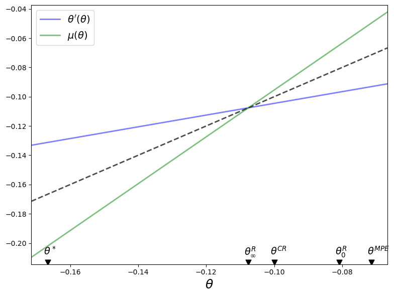
The dotted line in the above graph is the 45-degree line.

The blue line shows the choice of $\theta_{t+1} = \theta'$ chosen by a continuation Ramsey planner who inherits $\theta_t = \theta$.

The green line shows a continuation Ramsey planner’s choice of $\mu_t = \mu$ as a function of an inherited $\theta_t = \theta$.

Dynamics under the Ramsey plan are confined to $\theta \in \left[ \theta_\infty^R, \theta_0^R \right]$.

The blue and green lines intersect each other and the 45-degree line at $\theta =\theta_{\infty}^R$.

Notice that for $\theta \in \left(\theta_\infty^R, \theta_0^R \right]$

$\theta' < \theta$ because the blue line is below the 45-degree line
$\mu > \theta $ because the green line is above the 45-degree line

It follows that under the Ramsey plan $\{\theta_t\}$ and $\{\mu_t\}$ both converge monotonically from above to $\theta_\infty^R$.

The next code plots the Ramsey planner’s value function $J(\theta)$.

We know that $J (\theta)$ is maximized at $\theta^R_0$, the best time $0$ promised inflation rate.

The figure also plots the limiting value $\theta_\infty^R$, the limiting value of promised inflation rate $\theta_t$ under the Ramsey plan as $t \rightarrow +\infty$.

The figure also indicates an MPE inflation rate $\theta^{MPE}$, the inflation $\theta^{CR}$ under a Ramsey plan constrained to a constant money creation rate, and a bliss inflation $\theta^*$.

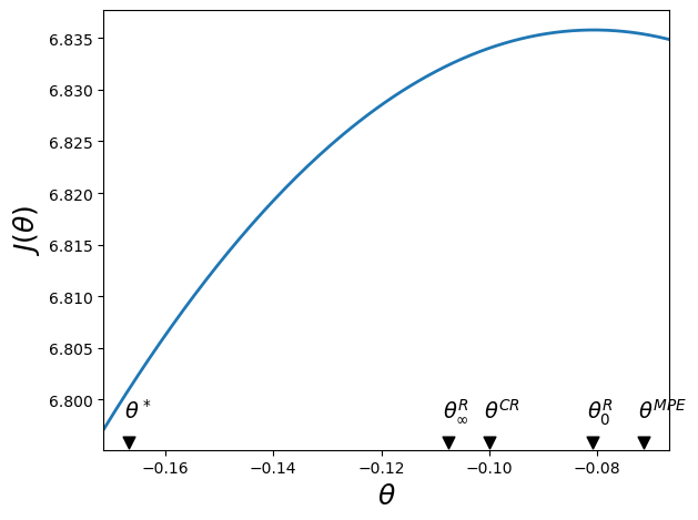
_images/ac18a0e46d965b6fdd77de6c20bdec35585771f7bad1ce59ef14e9d636a3818e.png

In the above graph, notice that $\theta^* < \theta_\infty^R < \theta^{CR} < \theta_0^R < \theta^{MPE}$:

$\theta_0^R < \theta^{MPE} $: the initial Ramsey inflation rate exceeds the MPE inflation rate
$\theta_\infty^R < \theta^{CR} <\theta_0^R$: the initial Ramsey deflation rate, and the associated tax distortion cost $c \mu_0^2$ is less than the limiting Ramsey inflation rate $\theta_\infty^R$ and the associated tax distortion cost $\mu_\infty^2$
$\theta^* < \theta^R_\infty$: the limiting Ramsey inflation rate exceeds the bliss level of inflation

In some subsequent calculations, we’ll use our Python code to study how gaps between these outcome vary depending on parameters such as the cost parameter $c$ and the discount factor $\beta$.

43.15. Ramsey Planner’s Value Function#

The next code plots the Ramsey Planner’s value function $J(\theta)$ as well as the value function of a constrained Ramsey planner who must choose a constant $\mu$.

A time-invariant $\mu$ implies a time-invariant $\theta$, we take the liberty of labeling this value function $V(\theta)$.

We’ll use the code to plot $J(\theta)$ and $V(\theta)$ for several values of the discount factor $\beta$ and the cost parameter $c$ that multiplies $\mu_t^2$ in the Ramsey planner’s one-period payoff function.

In all of the graphs below, we disarm the Proposition 1 equivalence results by setting $c >0$.

The graphs reveal interesting relationships among $\theta$’s associated with various timing protocols:

$J(\theta) \geq V(\theta)$
$J(\theta_\infty^R) = V(\theta_\infty^R)$

Before doing anything else, let’s write code to verify our claim that $J(\theta_\infty^R) = V(\theta_\infty^R)$.

Here is the code.

θ_inf = clq.θ_series[1, -1]
np.allclose(clq.J_θ(θ_inf),
            clq.V_θ(θ_inf))

True

So we have verified our claim that $J(\theta_\infty^R) = V(\theta_\infty^R)$.

Since $J(\theta_\infty^R) = V(\theta_\infty^R)$ occurs at a tangency point at which $J(\theta)$ is increasing in $\theta$, it follows that

(43.33)#\[ V(\theta_\infty^R) \leq J(\theta^{CR}) \]

with strict inequality when $c > 0$.

Thus, the value of the plan that sets the money growth rate $\mu_t = \theta_\infty^R$ for all $t \geq 0$ is worse than the value attained by a Ramsey planner who is constrained to set a constant $\mu_t$.

Now let’s write some code to plot outcomes under our three timing protocols.

For some default parameter values, the next figure plots the Ramsey planner’s continuation value function $J(\theta)$ (orange curve) and the restricted-to-constant-$\mu$ Ramsey planner’s value function $V(\theta)$ (blue curve).

The figure uses colored arrows to indicate locations of $\theta^*, \theta_\infty^R, \theta^{CR}, \theta_0^R$, and $\theta^{MPE}$, ordered as they are from left to right, on the $\theta$ axis.

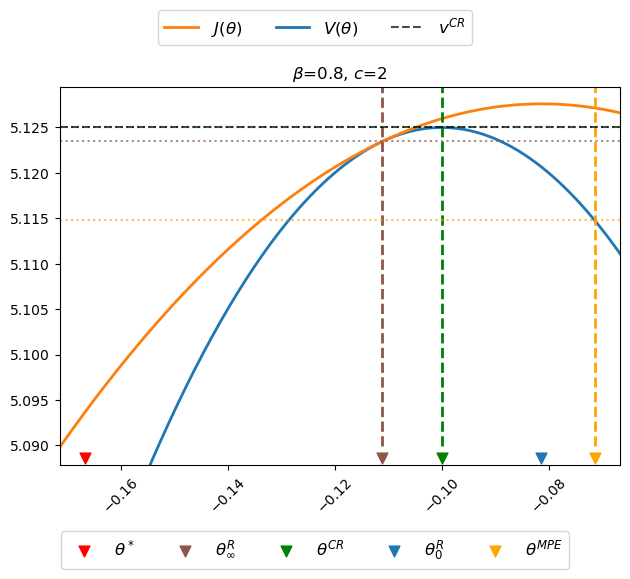
_images/ac9385d8976ec5ad5240570e0ea66950fd719d3dad8c1502058681dfb6965bbd.png

In the above figure, notice that

the orange $J$ value function lies above the blue $V$ value function except at $\theta = \theta_\infty^R$
the maximizer $\theta_0^R$ of $J(\theta)$ occurs at the top of the orange curve
the maximizer $\theta^{CR}$ of $V(\theta)$ occurs at the top of the blue curve
the “timeless perspective” inflation and money creation rate $\theta_\infty^R$ occurs where $J(\theta)$ is tangent to $V(\theta)$
the Markov perfect inflation and money creation rate $\theta^{MPE}$ exceeds $\theta_0^R$.
the value $V(\theta^{MPE})$ of the Markov perfect rate of money creation rate $\theta^{MPE}$ is less than the value $V(\theta_\infty^R)$ of the worst continuation Ramsey plan
the continuation value $J(\theta^{MPE})$ of the Markov perfect rate of money creation rate $\theta^{MPE}$ is greater than the value $V(\theta_\infty^R)$ and of the continuation value $J(\theta_\infty^R)$ of the worst continuation Ramsey plan

43.16. Perturbing Model Parameters#

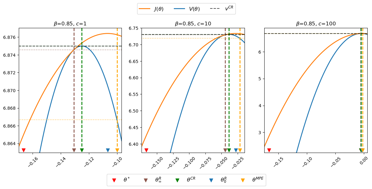
Now let’s present some graphs that teach us how outcomes change when we assume different values of $\beta$

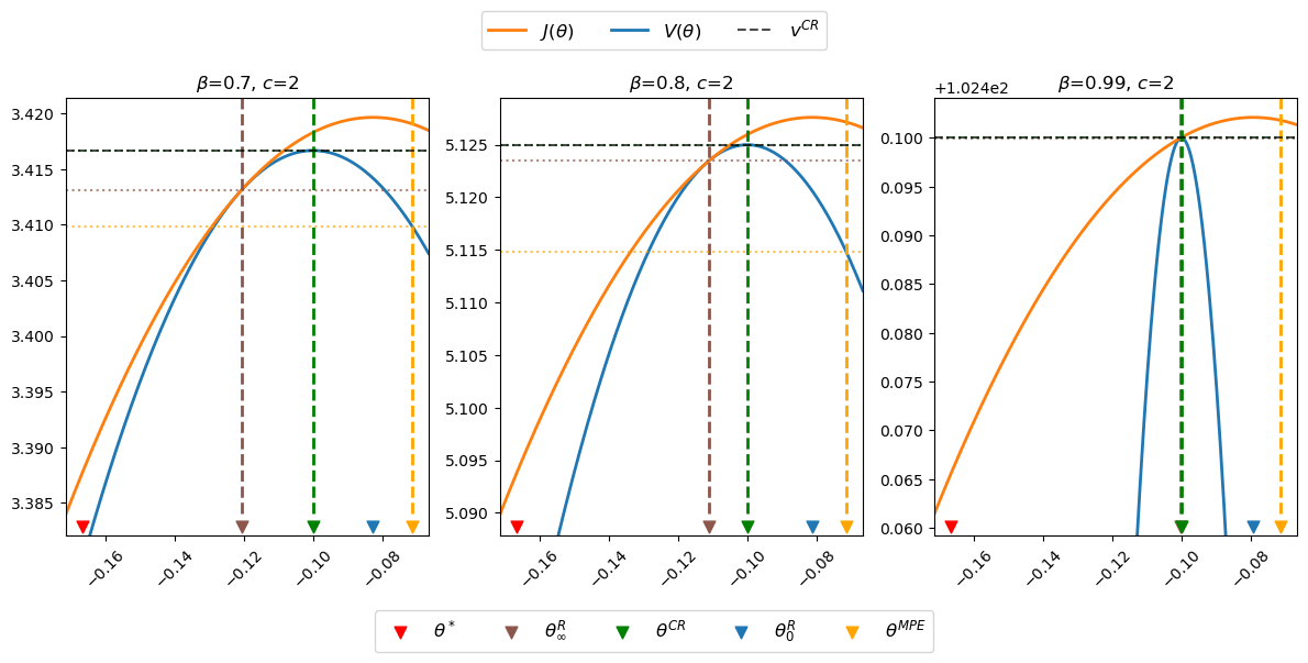
_images/7dc039726acba383ecdd4f1f121818c7da33afb0fe82012cd65e4bf8a4af9913.png

The horizontal dotted lines indicate values $V(\mu_\infty^R), V(\mu^{CR}), V(\mu^{MPE}) $ of time-invariant money growth rates $\mu_\infty^R, \mu^{CR}$ and $\mu^{MPE}$, respectfully.

Notice how $J(\theta)$ and $V(\theta)$ are tangent and increasing at $\theta = \theta_\infty^R$, which implies that $\theta^{CR} > \theta_\infty^R$ and $J(\theta^{CR}) > J(\theta_\infty^R)$.

Notice how changes in $\beta$ alter $\theta_\infty^R$ and $\theta_0^R$ but neither $\theta^*, \theta^{CR}$, nor $\theta^{MPE}$, in accord with formulas (43.8), (43.26), and (43.31), which imply that

\[\begin{split} \begin{aligned} \theta^{CR} & = - \frac{\alpha u_1}{\alpha^2 u_2 + c } \\ \theta^{MPE} & = - \frac{\alpha u_1}{\alpha^2 u_2 + (1+\alpha)c} \\ \theta^{*} & = -\frac{u_1}{u_2 \alpha} \end{aligned} \end{split}\]

The following table summarizes some outcomes.

\[\begin{split}\displaystyle \begin{array}{cccc} & \text{$\beta=0.7, c=2$} & \text{$\beta=0.8, c=2$} & \text{$\beta=0.99, c=2$} \\ \hline \text{$\theta^*$} & -0.167 & -0.167 & -0.167 \\ \text{$\theta_\infty^R$} & -0.121 & -0.111 & -0.100 \\ \text{$\theta^{CR}$} & -0.100 & -0.100 & -0.100 \\ \text{$\theta_0^R$} & -0.083 & -0.081 & -0.079 \\ \text{$\theta^{MPE}$} & -0.071 & -0.071 & -0.071 \end{array} \end{split}\]

But let’s see what happens when we change $c$.

# Increase c to 100
fig, axes = plt.subplots(1, 3, figsize=(12, 5))
c_values = [1, 10, 100]

clqs = [ChangLQ(β=0.85, c=c) for c in c_values]
plt_clqs(clqs, axes)

_images/c0c03dbba79e7fd96db1fc26931aa3041816a3f8d2d55bb95ebdcb3eaaa29bcb.png

generate_table(clqs, dig=4)

\[\begin{split}\displaystyle \begin{array}{cccc} & \text{$\beta=0.85, c=1$} & \text{$\beta=0.85, c=10$} & \text{$\beta=0.85, c=100$} \\ \hline \text{$\theta^*$} & -0.167 & -0.167 & -0.167 \\ \text{$\theta_\infty^R$} & -0.131 & -0.044 & -0.006 \\ \text{$\theta^{CR}$} & -0.125 & -0.038 & -0.005 \\ \text{$\theta_0^R$} & -0.107 & -0.028 & -0.003 \\ \text{$\theta^{MPE}$} & -0.100 & -0.022 & -0.003 \end{array} \end{split}\]

The above table and figures show how changes in $c$ alter $\theta_\infty^R$ and $\theta_0^R$ as well as $\theta^{CR}$ and $\theta^{MPE}$, but not $\theta^*,$ again in accord with formulas (43.8), (43.26), and (43.31).

Notice that as $c $ gets larger and larger, $\theta_\infty^R, \theta_0^R$ and $\theta^{CR}$ all converge to $\theta^{MPE}$.

Now let’s watch what happens when we drive $c$ toward zero.

# Decrease c towards 0
fig, axes = plt.subplots(1, 3, figsize=(12, 5))
c_limits = [1, 0.1, 0.01]

clqs = [ChangLQ(β=0.85, c=c) for c in c_limits]
plt_clqs(clqs, axes)

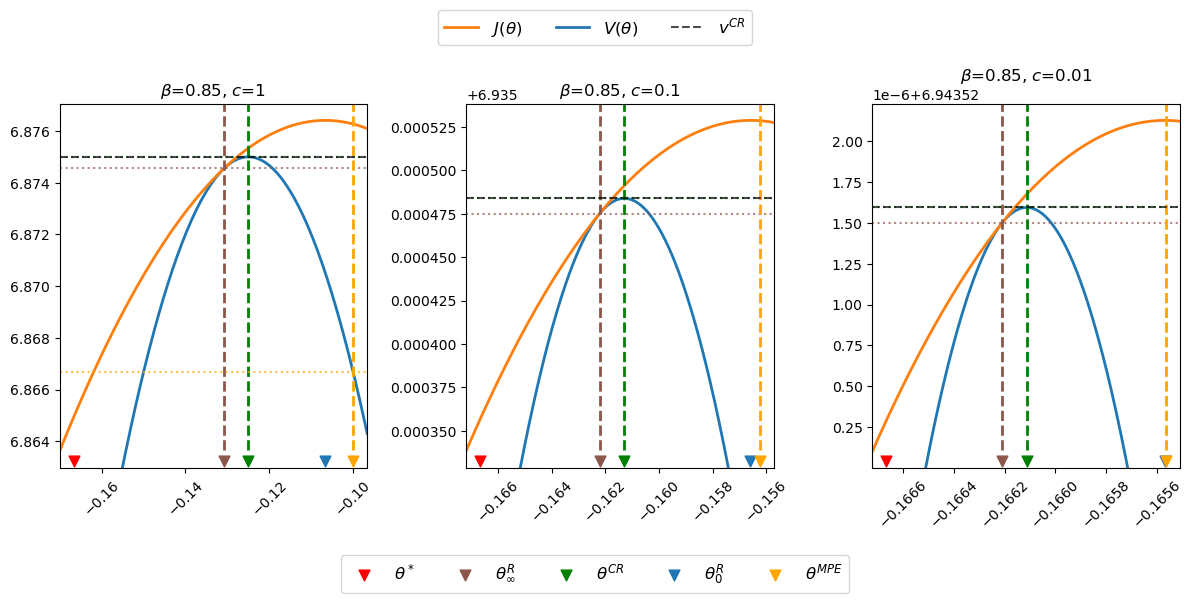
_images/c68331e98a0547f1f0bf42a8999ea7078cc9269963b7d804442b74d4771d308b.png

The above graphs indicate that as $c$ approaches zero, $\theta_\infty^R, \theta_0^R, \theta^{CR}$, and $\theta^{MPE}$ all approach $\theta^*$.

This makes sense, because it was by adding costs of distorting taxes that Calvo [Calvo, 1978] drove a wedge between Friedman’s optimal deflation rate and the inflation rates chosen by a Ramsey planner.

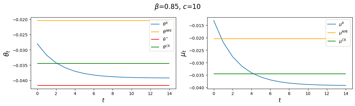
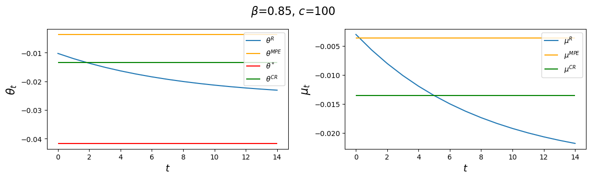
The following code plots sequences $\vec \mu$ and $\vec \theta$ prescribed by a Ramsey plan as well as the constant levels $\mu^{CR}$ and $\mu^{MPE}$.

The following graphs report values for the value function parameters $g_0, g_1, g_2$, and the Ramsey policy function parameters $b_0, b_1, d_0, d_1$ associated with the indicated parameter pair $\beta, c$.

We’ll vary $\beta$ while keeping a small $c$.

After that we’ll study consequences of raising $c$.

We’ll watch how the decay rate $d_1$ governing the dynamics of $\theta_t^R$ is affected by alterations in the parameters $\beta, c$.

for β in β_values:
    clq = ChangLQ(β=β, c=2)
    generate_param_table(clq)
    plot_ramsey_MPE(clq)

\[\begin{split}\displaystyle \begin{array}{cccccccc} & \text{$g_0$} & \text{$g_1$} & \text{$g_2$} & \text{$b_0$} & \text{$b_1$} & \text{$d_0$} & \text{$d_1$} \\ \hline \text{$\beta=0.7, c=2$} & 3.39 & -0.75 & -4.54 & -0.06 & -1.52 & -0.06 & 0.48 \end{array} \end{split}\]

_images/577973641b911c3502157ed6405d8d99f8a42bc0bf46ec5d2865be66650d10fe.png

\[\begin{split}\displaystyle \begin{array}{cccccccc} & \text{$g_0$} & \text{$g_1$} & \text{$g_2$} & \text{$b_0$} & \text{$b_1$} & \text{$d_0$} & \text{$d_1$} \\ \hline \text{$\beta=0.8, c=2$} & 5.1 & -0.76 & -4.65 & -0.06 & -1.58 & -0.06 & 0.42 \end{array} \end{split}\]

_images/0379a4da55825adbc12fdfbd056cec7fffa7c1395664784a68a3152400ae28e2.png

\[\begin{split}\displaystyle \begin{array}{cccccccc} & \text{$g_0$} & \text{$g_1$} & \text{$g_2$} & \text{$b_0$} & \text{$b_1$} & \text{$d_0$} & \text{$d_1$} \\ \hline \text{$\beta=0.99, c=2$} & 102.47 & -0.76 & -4.81 & -0.07 & -1.65 & -0.07 & 0.35 \end{array} \end{split}\]

_images/242396dce0a867e8847676bebaea59375ab59ae2b4409c0b84040529cc6412e9.png

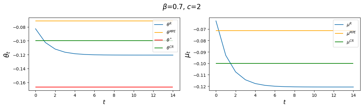
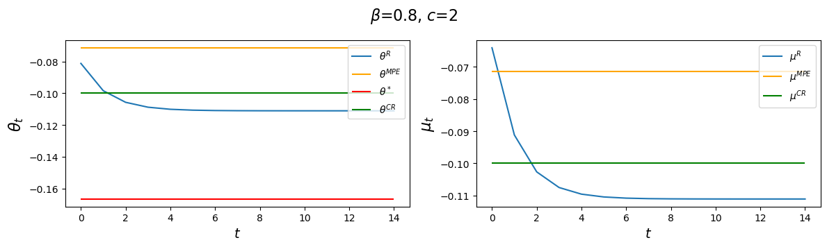
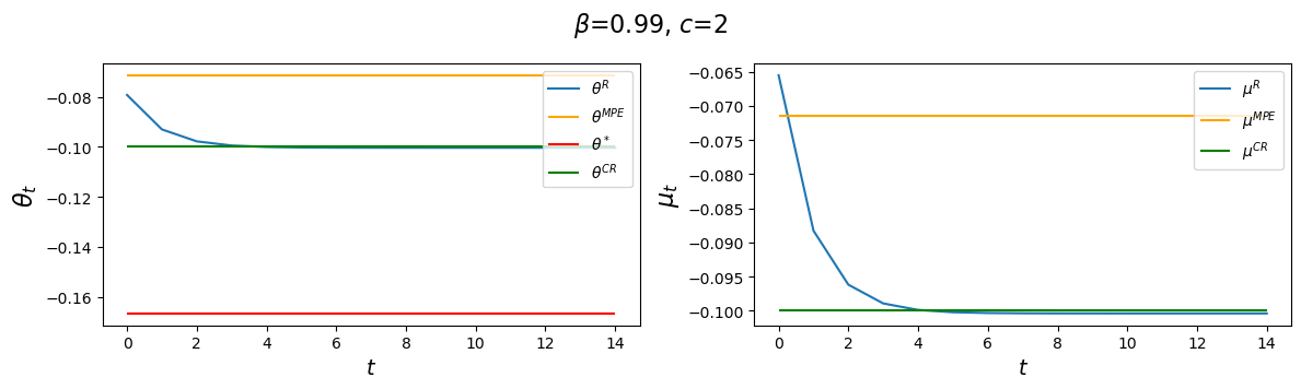
Notice how $d_1$ changes as we raise the discount factor parameter $\beta$.

Now let’s study how increasing $c$ affects $\vec \theta, \vec \mu$ outcomes.

# Increase c to 100
for c in c_values:
    clq = ChangLQ(β=0.85, c=c)
    generate_param_table(clq)
    plot_ramsey_MPE(clq)

\[\begin{split}\displaystyle \begin{array}{cccccccc} & \text{$g_0$} & \text{$g_1$} & \text{$g_2$} & \text{$b_0$} & \text{$b_1$} & \text{$d_0$} & \text{$d_1$} \\ \hline \text{$\beta=0.85, c=1$} & 6.84 & -0.68 & -3.19 & -0.09 & -1.69 & -0.09 & 0.31 \end{array} \end{split}\]

_images/8904591562597e73a2721b5a34c499b5ab3c3ca2942b273b96c4883d3fcf7ff5.png

\[\begin{split}\displaystyle \begin{array}{cccccccc} & \text{$g_0$} & \text{$g_1$} & \text{$g_2$} & \text{$b_0$} & \text{$b_1$} & \text{$d_0$} & \text{$d_1$} \\ \hline \text{$\beta=0.85, c=10$} & 6.72 & -0.92 & -16.16 & -0.02 & -1.47 & -0.02 & 0.53 \end{array} \end{split}\]

_images/7fb469b87ca9b95c3cea09fdb74385b04d781fedb921719382602d327cd1c3fe.png

\[\begin{split}\displaystyle \begin{array}{cccccccc} & \text{$g_0$} & \text{$g_1$} & \text{$g_2$} & \text{$b_0$} & \text{$b_1$} & \text{$d_0$} & \text{$d_1$} \\ \hline \text{$\beta=0.85, c=100$} & 6.67 & -0.99 & -143.29 & -0.0 & -1.42 & -0.0 & 0.58 \end{array} \end{split}\]

_images/3703953e40f16553c7a69bdc2cdec0ce21c9092042501bc872707757d4ba33a4.png

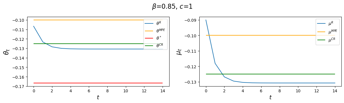
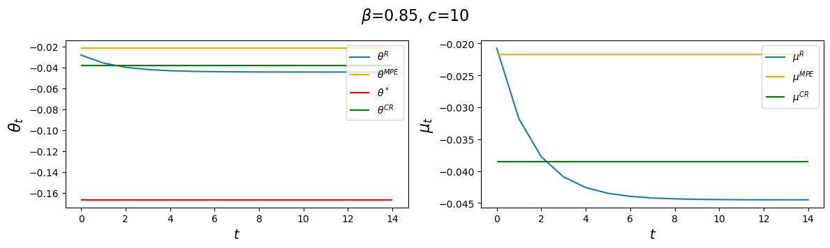
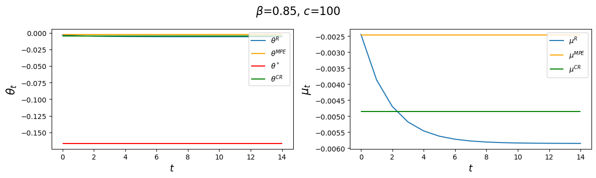
Evidently, increasing $c$ causes the decay factor $d_1$ to increase.

Next, let’s look at consequences of increasing the demand for real balances parameter $\alpha$ from its default value $\alpha=1$ to $\alpha=4$.

# Increase c to 100
for c in [10, 100]:
    clq = ChangLQ(α=4, β=0.85, c=c)
    generate_param_table(clq)
    plot_ramsey_MPE(clq)

\[\begin{split}\displaystyle \begin{array}{cccccccc} & \text{$g_0$} & \text{$g_1$} & \text{$g_2$} & \text{$b_0$} & \text{$b_1$} & \text{$d_0$} & \text{$d_1$} \\ \hline \text{$\beta=0.85, c=10$} & 6.84 & -4.62 & -82.32 & -0.05 & -2.33 & -0.01 & 0.67 \end{array} \end{split}\]

_images/0208c7e0713fd1b094fdcca27199163f73ad16794ba227fb627f722daed8c7de.png

\[\begin{split}\displaystyle \begin{array}{cccccccc} & \text{$g_0$} & \text{$g_1$} & \text{$g_2$} & \text{$b_0$} & \text{$b_1$} & \text{$d_0$} & \text{$d_1$} \\ \hline \text{$\beta=0.85, c=100$} & 6.74 & -8.03 & -390.65 & -0.01 & -1.47 & -0.0 & 0.88 \end{array} \end{split}\]

_images/2a74e28ca8f69f626cb26613624426d8b8d4fd531db8028cd57e455aded7b4c3.png

The above panels for an $\alpha = 4$ setting indicate that $\alpha$ and $c$ affect outcomes in interesting ways.

We leave it to the reader to explore consequences of other constellations of parameter values.

43.16.1. Implausibility of Ramsey Plan#

Many economists regard a time inconsistent plan as implausible because they question the plausibility of timing protocol in which a plan for setting a sequence of policy variables is chosen once-and-for-all at time $0$.

For that reason, the Markov perfect equilibrium concept attracts many economists.

A Markov perfect equilibrium plan is constructed to insure that a sequence of government policymakers who choose sequentially do not want to deviate from it.

43.16.2. Ramsey Plan Strikes Back#

Research by Abreu [Abreu, 1988], Chari and Kehoe [Chari and Kehoe, 1990] [Stokey, 1989], and Stokey [Stokey, 1991] described conditions under which a Ramsey plan can be rescued from the complaint that it is not credible.

They accomplished this by expanding the description of a plan to include expectations about adverse consequences of deviating from it that can serve to deter deviations.

We turn to such theories in this quantecon lecture Sustainable Plans for a Calvo Model.

43. Time Inconsistency of Ramsey Plans#

43.1. Overview#

43.2. Model Components#

43.3. Friedman’s Optimal Rate of Deflation#

43.4. Calvo’s Distortion#

43.5. Structure#

43.5.1. Intertemporal Aspects#

43.6. Three Timing Protocols#

43.7. Note on Dynamic Programming Squared#

43.8. A Ramsey Planner#

43.8.1. Subproblem 1#

43.8.2. Subproblem 2#

43.9. Representation of Ramsey Plan#

43.10. Multiple roles of \(\theta_t\)#

43.11. Time inconsistency#

43.12. Constrained-to-Constant-Growth-Rate Ramsey Plan#

43.13. Markov Perfect Governments#

43.14. Outcomes under Three Timing Protocols#

43.15. Ramsey Planner’s Value Function#

43.16. Perturbing Model Parameters#

43.16.1. Implausibility of Ramsey Plan#

43.16.2. Ramsey Plan Strikes Back#