48. Fiscal Risk and Government Debt#

In addition to what’s in Anaconda, this lecture will need the following libraries:

!pip install --upgrade quantecon

48.1. Overview#

This lecture studies government debt in an AMSS economy [Aiyagari et al., 2002] of the type described in Optimal Taxation without State-Contingent Debt.

We study the behavior of government debt as time \(t \rightarrow + \infty\).

We use these techniques

simulations
a regression coefficient from the tail of a long simulation that allows us to verify that the asymptotic mean of government debt solves a fiscal-risk minimization problem
an approximation to the mean of an ergodic distribution of government debt
an approximation to the rate of convergence to an ergodic distribution of government debt

We apply tools that are applicable to more general incomplete markets economies that are presented on pages 648 - 650 in section III.D of [Bhandari et al., 2017] (BEGS).

We study an AMSS economy [Aiyagari et al., 2002] with three Markov states driving government expenditures.

In a previous lecture, we showed that with only two Markov states, it is possible that endogenous interest rate fluctuations eventually can support complete markets allocations and Ramsey outcomes.
The presence of three states prevents the full spanning that eventually prevails in the two-state example featured in Fiscal Insurance via Fluctuating Interest Rates.

The lack of full spanning means that the ergodic distribution of the par value of government debt is nontrivial, in contrast to the situation in Fiscal Insurance via Fluctuating Interest Rates in which the ergodic distribution of the par value of government debt is concentrated on one point.

Nevertheless, [Bhandari et al., 2017] (BEGS) establish that, for general settings that include ours, the Ramsey planner steers government assets to a level that comes as close as possible to providing full spanning in a precise a sense defined by BEGS that we describe below.

We use code constructed in Fluctuating Interest Rates Deliver Fiscal Insurance.

Warning: Key equations in [Bhandari et al., 2017] section III.D carry typos that we correct below.

Let’s start with some imports:

import matplotlib.pyplot as plt
from scipy.optimize import minimize

48.2. The Economy#

As in Optimal Taxation without State-Contingent Debt and Optimal Taxation with State-Contingent Debt, we assume that the representative agent has utility function

\[ u(c,n) = {\frac{c^{1-\sigma}}{1-\sigma}} - {\frac{n^{1+\gamma}}{1+\gamma}} \]

We work directly with labor supply instead of leisure.

We assume that

\[ c_t + g_t = n_t \]

The Markov state \(s_t\) takes three values, namely, \(0,1,2\).

The initial Markov state is \(0\).

The Markov transition matrix is \((1/3) I\) where \(I\) is a \(3 \times 3\) identity matrix, so the \(s_t\) process is IID.

Government expenditures \(g(s)\) equal \(.1\) in Markov state \(0\), \(.2\) in Markov state \(1\), and \(.3\) in Markov state \(2\).

We set preference parameters

\[ \begin{aligned} \beta & = .9 \cr \sigma & = 2 \cr \gamma & = 2 \end{aligned} \]

The following Python code sets up the economy

import numpy as np


class CRRAutility:

    def __init__(self,
                 β=0.9,
                 σ=2,
                 γ=2,
                 π=np.full((2, 2), 0.5),
                 G=np.array([0.1, 0.2]),
                 Θ=np.ones(2),
                 transfers=False):

        self.β, self.σ, self.γ = β, σ, γ
        self.π, self.G, self.Θ, self.transfers = π, G, Θ, transfers

    # Utility function
    def U(self, c, n):
        σ = self.σ
        if σ == 1.:
            U = np.log(c)
        else:
            U = (c**(1 - σ) - 1) / (1 - σ)
        return U - n**(1 + self.γ) / (1 + self.γ)

    # Derivatives of utility function
    def Uc(self, c, n):
        return c**(-self.σ)

    def Ucc(self, c, n):
        return -self.σ * c**(-self.σ - 1)

    def Un(self, c, n):
        return -n**self.γ

    def Unn(self, c, n):
        return -self.γ * n**(self.γ - 1)

48.2.1. First and Second Moments#

We’ll want first and second moments of some key random variables below.

The following code computes these moments; the code is recycled from Fluctuating Interest Rates Deliver Fiscal Insurance.

def mean(x, s):
    '''Returns mean for x given initial state'''
    x = np.array(x)
    return x @ u.π[s]

def variance(x, s):
    x = np.array(x)
    return x**2 @ u.π[s] - mean(x, s)**2

def covariance(x, y, s):
    x, y = np.array(x), np.array(y)
    return x * y @ u.π[s] - mean(x, s) * mean(y, s)

48.3. Long Simulation#

To generate a long simulation we use the following code.

We begin by showing the code that we used in earlier lectures on the AMSS model.

Here it is

import numpy as np
from scipy.optimize import root
from quantecon import MarkovChain


class SequentialAllocation:

    '''
    Class that takes CESutility or BGPutility object as input returns
    planner's allocation as a function of the multiplier on the
    implementability constraint μ.
    '''

    def __init__(self, model):

        # Initialize from model object attributes
        self.β, self.π, self.G = model.β, model.π, model.G
        self.mc, self.Θ = MarkovChain(self.π), model.Θ
        self.S = len(model.π)  # Number of states
        self.model = model

        # Find the first best allocation
        self.find_first_best()

    def find_first_best(self):
        '''
        Find the first best allocation
        '''
        model = self.model
        S, Θ, G = self.S, self.Θ, self.G
        Uc, Un = model.Uc, model.Un

        def res(z):
            c = z[:S]
            n = z[S:]
            return np.hstack([Θ * Uc(c, n) + Un(c, n), Θ * n - c - G])

        res = root(res, np.full(2 * S, 0.5))

        if not res.success:
            raise Exception('Could not find first best')

        self.cFB = res.x[:S]
        self.nFB = res.x[S:]

        # Multiplier on the resource constraint
        self.ΞFB = Uc(self.cFB, self.nFB)
        self.zFB = np.hstack([self.cFB, self.nFB, self.ΞFB])

    def time1_allocation(self, μ):
        '''
        Computes optimal allocation for time t >= 1 for a given μ
        '''
        model = self.model
        S, Θ, G = self.S, self.Θ, self.G
        Uc, Ucc, Un, Unn = model.Uc, model.Ucc, model.Un, model.Unn

        def FOC(z):
            c = z[:S]
            n = z[S:2 * S]
            Ξ = z[2 * S:]
            # FOC of c
            return np.hstack([Uc(c, n) - μ * (Ucc(c, n) * c + Uc(c, n)) - Ξ,
                              Un(c, n) - μ * (Unn(c, n) * n + Un(c, n)) \
                              + Θ * Ξ,  # FOC of n
                              Θ * n - c - G])

        # Find the root of the first-order condition
        res = root(FOC, self.zFB)
        if not res.success:
            raise Exception('Could not find LS allocation.')
        z = res.x
        c, n, Ξ = z[:S], z[S:2 * S], z[2 * S:]

        # Compute x
        I = Uc(c, n) * c + Un(c, n) * n
        x = np.linalg.solve(np.eye(S) - self.β * self.π, I)

        return c, n, x, Ξ

    def time0_allocation(self, B_, s_0):
        '''
        Finds the optimal allocation given initial government debt B_ and
        state s_0
        '''
        model, π, Θ, G, β = self.model, self.π, self.Θ, self.G, self.β
        Uc, Ucc, Un, Unn = model.Uc, model.Ucc, model.Un, model.Unn

        # First order conditions of planner's problem
        def FOC(z):
            μ, c, n, Ξ = z
            xprime = self.time1_allocation(μ)[2]
            return np.hstack([Uc(c, n) * (c - B_) + Un(c, n) * n + β * π[s_0]
                                            @ xprime,
                              Uc(c, n) - μ * (Ucc(c, n)
                                            * (c - B_) + Uc(c, n)) - Ξ,
                              Un(c, n) - μ * (Unn(c, n) * n
                                            + Un(c, n)) + Θ[s_0] * Ξ,
                              (Θ * n - c - G)[s_0]])

        # Find root
        res = root(FOC, np.array(
            [0, self.cFB[s_0], self.nFB[s_0], self.ΞFB[s_0]]))
        if not res.success:
            raise Exception('Could not find time 0 LS allocation.')

        return res.x

    def time1_value(self, μ):
        '''
        Find the value associated with multiplier μ
        '''
        c, n, x, Ξ = self.time1_allocation(μ)
        U = self.model.U(c, n)
        V = np.linalg.solve(np.eye(self.S) - self.β * self.π, U)
        return c, n, x, V

    def Τ(self, c, n):
        '''
        Computes Τ given c, n
        '''
        model = self.model
        Uc, Un = model.Uc(c, n), model.Un(c,  n)

        return 1 + Un / (self.Θ * Uc)

    def simulate(self, B_, s_0, T, sHist=None):
        '''
        Simulates planners policies for T periods
        '''
        model, π, β = self.model, self.π, self.β
        Uc = model.Uc

        if sHist is None:
            sHist = self.mc.simulate(T, s_0)

        cHist, nHist, Bhist, ΤHist, μHist = np.zeros((5, T))
        RHist = np.zeros(T - 1)

        # Time 0
        μ, cHist[0], nHist[0], _ = self.time0_allocation(B_, s_0)
        ΤHist[0] = self.Τ(cHist[0], nHist[0])[s_0]
        Bhist[0] = B_
        μHist[0] = μ

        # Time 1 onward
        for t in range(1, T):
            c, n, x, Ξ = self.time1_allocation(μ)
            Τ = self.Τ(c, n)
            u_c = Uc(c, n)
            s = sHist[t]
            Eu_c = π[sHist[t - 1]] @ u_c
            cHist[t], nHist[t], Bhist[t], ΤHist[t] = c[s], n[s], x[s] / u_c[s], \
                                                     Τ[s]
            RHist[t - 1] = Uc(cHist[t - 1], nHist[t - 1]) / (β * Eu_c)
            μHist[t] = μ

        return [cHist, nHist, Bhist, ΤHist, sHist, μHist, RHist]

import numpy as np
from scipy.optimize import fmin_slsqp
from scipy.optimize import root
from quantecon import MarkovChain


class RecursiveAllocationAMSS:

    def __init__(self, model, μgrid, tol_diff=1e-7, tol=1e-7):

        self.β, self.π, self.G = model.β, model.π, model.G
        self.mc, self.S = MarkovChain(self.π), len(model.π)  # Number of states
        self.Θ, self.model, self.μgrid = model.Θ, model, μgrid
        self.tol_diff, self.tol = tol_diff, tol

        # Find the first best allocation
        self.solve_time1_bellman()
        self.T.time_0 = True  # Bellman equation now solves time 0 problem

    def solve_time1_bellman(self):
        '''
        Solve the time  1 Bellman equation for calibration model and
        initial grid μgrid0
        '''
        model, μgrid0 = self.model, self.μgrid
        π = model.π
        S = len(model.π)

        # First get initial fit from Lucas Stokey solution.
        # Need to change things to be ex ante
        pp = SequentialAllocation(model)
        interp = interpolator_factory(2, None)

        def incomplete_allocation(μ_, s_):
            c, n, x, V = pp.time1_value(μ_)
            return c, n, π[s_] @ x, π[s_] @ V
        cf, nf, xgrid, Vf, xprimef = [], [], [], [], []
        for s_ in range(S):
            c, n, x, V = zip(*map(lambda μ: incomplete_allocation(μ, s_), μgrid0))
            c, n = np.vstack(c).T, np.vstack(n).T
            x, V = np.hstack(x), np.hstack(V)
            xprimes = np.vstack([x] * S)
            cf.append(interp(x, c))
            nf.append(interp(x, n))
            Vf.append(interp(x, V))
            xgrid.append(x)
            xprimef.append(interp(x, xprimes))
        cf, nf, xprimef = fun_vstack(cf), fun_vstack(nf), fun_vstack(xprimef)
        Vf = fun_hstack(Vf)
        policies = [cf, nf, xprimef]

        # Create xgrid
        x = np.vstack(xgrid).T
        xbar = [x.min(0).max(), x.max(0).min()]
        xgrid = np.linspace(xbar[0], xbar[1], len(μgrid0))
        self.xgrid = xgrid

        # Now iterate on Bellman equation
        T = BellmanEquation(model, xgrid, policies, tol=self.tol)
        diff = 1
        while diff > self.tol_diff:
            PF = T(Vf)

            Vfnew, policies = self.fit_policy_function(PF)
            diff = np.abs((Vf(xgrid) - Vfnew(xgrid)) / Vf(xgrid)).max()

            print(diff)
            Vf = Vfnew

        # Store value function policies and Bellman Equations
        self.Vf = Vf
        self.policies = policies
        self.T = T

    def fit_policy_function(self, PF):
        '''
        Fits the policy functions
        '''
        S, xgrid = len(self.π), self.xgrid
        interp = interpolator_factory(3, 0)
        cf, nf, xprimef, Tf, Vf = [], [], [], [], []
        for s_ in range(S):
            PFvec = np.vstack([PF(x, s_) for x in self.xgrid]).T
            Vf.append(interp(xgrid, PFvec[0, :]))
            cf.append(interp(xgrid, PFvec[1:1 + S]))
            nf.append(interp(xgrid, PFvec[1 + S:1 + 2 * S]))
            xprimef.append(interp(xgrid, PFvec[1 + 2 * S:1 + 3 * S]))
            Tf.append(interp(xgrid, PFvec[1 + 3 * S:]))
        policies = fun_vstack(cf), fun_vstack(
            nf), fun_vstack(xprimef), fun_vstack(Tf)
        Vf = fun_hstack(Vf)
        return Vf, policies

    def Τ(self, c, n):
        '''
        Computes Τ given c and n
        '''
        model = self.model
        Uc, Un = model.Uc(c, n), model.Un(c, n)

        return 1 + Un / (self.Θ * Uc)

    def time0_allocation(self, B_, s0):
        '''
        Finds the optimal allocation given initial government debt B_ and
        state s_0
        '''
        PF = self.T(self.Vf)
        z0 = PF(B_, s0)
        c0, n0, xprime0, T0 = z0[1:]
        return c0, n0, xprime0, T0

    def simulate(self, B_, s_0, T, sHist=None):
        '''
        Simulates planners policies for T periods
        '''
        model, π = self.model, self.π
        Uc = model.Uc
        cf, nf, xprimef, Tf = self.policies

        if sHist is None:
            sHist = simulate_markov(π, s_0, T)

        cHist, nHist, Bhist, xHist, ΤHist, THist, μHist = np.zeros((7, T))
        # Time 0
        cHist[0], nHist[0], xHist[0], THist[0] = self.time0_allocation(B_, s_0)
        ΤHist[0] = self.Τ(cHist[0], nHist[0])[s_0]
        Bhist[0] = B_
        μHist[0] = self.Vf[s_0](xHist[0])

        # Time 1 onward
        for t in range(1, T):
            s_, x, s = sHist[t - 1], xHist[t - 1], sHist[t]
            c, n, xprime, T = cf[s_, :](x), nf[s_, :](
                x), xprimef[s_, :](x), Tf[s_, :](x)

            Τ = self.Τ(c, n)[s]
            u_c = Uc(c, n)
            Eu_c = π[s_, :] @ u_c

            μHist[t] = self.Vf[s](xprime[s])

            cHist[t], nHist[t], Bhist[t], ΤHist[t] = c[s], n[s], x / Eu_c, Τ
            xHist[t], THist[t] = xprime[s], T[s]
        return [cHist, nHist, Bhist, ΤHist, THist, μHist, sHist, xHist]


class BellmanEquation:
    '''
    Bellman equation for the continuation of the Lucas-Stokey Problem
    '''

    def __init__(self, model, xgrid, policies0, tol, maxiter=1000):

        self.β, self.π, self.G = model.β, model.π, model.G
        self.S = len(model.π)  # Number of states
        self.Θ, self.model, self.tol = model.Θ, model, tol
        self.maxiter = maxiter

        self.xbar = [min(xgrid), max(xgrid)]
        self.time_0 = False

        self.z0 = {}
        cf, nf, xprimef = policies0

        for s_ in range(self.S):
            for x in xgrid:
                self.z0[x, s_] = np.hstack([cf[s_, :](x),
                                            nf[s_, :](x),
                                            xprimef[s_, :](x),
                                            np.zeros(self.S)])

        self.find_first_best()

    def find_first_best(self):
        '''
        Find the first best allocation
        '''
        model = self.model
        S, Θ, Uc, Un, G = self.S, self.Θ, model.Uc, model.Un, self.G

        def res(z):
            c = z[:S]
            n = z[S:]
            return np.hstack([Θ * Uc(c, n) + Un(c, n), Θ * n - c - G])

        res = root(res, np.full(2 * S, 0.5))
        if not res.success:
            raise Exception('Could not find first best')

        self.cFB = res.x[:S]
        self.nFB = res.x[S:]
        IFB = Uc(self.cFB, self.nFB) * self.cFB + \
            Un(self.cFB, self.nFB) * self.nFB

        self.xFB = np.linalg.solve(np.eye(S) - self.β * self.π, IFB)

        self.zFB = {}
        for s in range(S):
            self.zFB[s] = np.hstack(
                [self.cFB[s], self.nFB[s], self.π[s] @ self.xFB, 0.])

    def __call__(self, Vf):
        '''
        Given continuation value function next period return value function this
        period return T(V) and optimal policies
        '''
        if not self.time_0:
            def PF(x, s): return self.get_policies_time1(x, s, Vf)
        else:
            def PF(B_, s0): return self.get_policies_time0(B_, s0, Vf)
        return PF

    def get_policies_time1(self, x, s_, Vf):
        '''
        Finds the optimal policies 
        '''
        model, β, Θ, G, S, π = self.model, self.β, self.Θ, self.G, self.S, self.π
        U, Uc, Un = model.U, model.Uc, model.Un

        def objf(z):
            c, n, xprime = z[:S], z[S:2 * S], z[2 * S:3 * S]

            Vprime = np.empty(S)
            for s in range(S):
                Vprime[s] = Vf[s](xprime[s])

            return -π[s_] @ (U(c, n) + β * Vprime)

        def objf_prime(x):

            epsilon = 1e-7
            x0 = np.asfarray(x)
            f0 = np.atleast_1d(objf(x0))
            jac = np.zeros([len(x0), len(f0)])
            dx = np.zeros(len(x0))
            for i in range(len(x0)):
                dx[i] = epsilon
                jac[i] = (objf(x0+dx) - f0)/epsilon
                dx[i] = 0.0

            return jac.transpose()

        def cons(z):
            c, n, xprime, T = z[:S], z[S:2 * S], z[2 * S:3 * S], z[3 * S:]
            u_c = Uc(c, n)
            Eu_c = π[s_] @ u_c
            return np.hstack([
                x * u_c / Eu_c - u_c * (c - T) - Un(c, n) * n - β * xprime,
                Θ * n - c - G])

        if model.transfers:
            bounds = [(0., 100)] * S + [(0., 100)] * S + \
                [self.xbar] * S + [(0., 100.)] * S
        else:
            bounds = [(0., 100)] * S + [(0., 100)] * S + \
                [self.xbar] * S + [(0., 0.)] * S
        out, fx, _, imode, smode = fmin_slsqp(objf, self.z0[x, s_],
                                              f_eqcons=cons, bounds=bounds,
                                              fprime=objf_prime, full_output=True,
                                              iprint=0, acc=self.tol, iter=self.maxiter)

        if imode > 0:
            raise Exception(smode)

        self.z0[x, s_] = out
        return np.hstack([-fx, out])

    def get_policies_time0(self, B_, s0, Vf):
        '''
        Finds the optimal policies 
        '''
        model, β, Θ, G = self.model, self.β, self.Θ, self.G
        U, Uc, Un = model.U, model.Uc, model.Un

        def objf(z):
            c, n, xprime = z[:-1]

            return -(U(c, n) + β * Vf[s0](xprime))

        def cons(z):
            c, n, xprime, T = z
            return np.hstack([
                -Uc(c, n) * (c - B_ - T) - Un(c, n) * n - β * xprime,
                (Θ * n - c - G)[s0]])

        if model.transfers:
            bounds = [(0., 100), (0., 100), self.xbar, (0., 100.)]
        else:
            bounds = [(0., 100), (0., 100), self.xbar, (0., 0.)]
        out, fx, _, imode, smode = fmin_slsqp(objf, self.zFB[s0], f_eqcons=cons,
                                              bounds=bounds, full_output=True,
                                              iprint=0)

        if imode > 0:
            raise Exception(smode)

        return np.hstack([-fx, out])

import numpy as np
from scipy.interpolate import UnivariateSpline


class interpolate_wrapper:

    def __init__(self, F):
        self.F = F

    def __getitem__(self, index):
        return interpolate_wrapper(np.asarray(self.F[index]))

    def reshape(self, *args):
        self.F = self.F.reshape(*args)
        return self

    def transpose(self):
        self.F = self.F.transpose()

    def __len__(self):
        return len(self.F)

    def __call__(self, xvec):
        x = np.atleast_1d(xvec)
        shape = self.F.shape
        if len(x) == 1:
            fhat = np.hstack([f(x) for f in self.F.flatten()])
            return fhat.reshape(shape)
        else:
            fhat = np.vstack([f(x) for f in self.F.flatten()])
            return fhat.reshape(np.hstack((shape, len(x))))


class interpolator_factory:

    def __init__(self, k, s):
        self.k, self.s = k, s

    def __call__(self, xgrid, Fs):
        shape, m = Fs.shape[:-1], Fs.shape[-1]
        Fs = Fs.reshape((-1, m))
        F = []
        xgrid = np.sort(xgrid)  # Sort xgrid
        for Fhat in Fs:
            F.append(UnivariateSpline(xgrid, Fhat, k=self.k, s=self.s))
        return interpolate_wrapper(np.array(F).reshape(shape))


def fun_vstack(fun_list):

    Fs = [IW.F for IW in fun_list]
    return interpolate_wrapper(np.vstack(Fs))


def fun_hstack(fun_list):

    Fs = [IW.F for IW in fun_list]
    return interpolate_wrapper(np.hstack(Fs))


def simulate_markov(π, s_0, T):

    sHist = np.empty(T, dtype=int)
    sHist[0] = s_0
    S = len(π)
    for t in range(1, T):
        sHist[t] = np.random.choice(np.arange(S), p=π[sHist[t - 1]])

    return sHist

Next, we show the code that we use to generate a very long simulation starting from initial government debt equal to \(-.5\).

Here is a graph of a long simulation of 102000 periods.

μ_grid = np.linspace(-0.09, 0.1, 100)

log_example = CRRAutility(π=np.full((3, 3), 1 / 3),
                          G=np.array([0.1, 0.2, .3]),
                          Θ=np.ones(3))

log_example.transfers = True        # Government can use transfers
log_sequential = SequentialAllocation(log_example)  # Solve sequential problem
log_bellman = RecursiveAllocationAMSS(log_example, μ_grid,
                                       tol=1e-12, tol_diff=1e-10)



T = 102000  # Set T to 102000 periods

sim_seq_long = log_sequential.simulate(0.5, 0, T)
sHist_long = sim_seq_long[-3]
sim_bel_long = log_bellman.simulate(0.5, 0, T, sHist_long)

titles = ['Government Debt', 'Tax Rate']

fig, axes = plt.subplots(2, 1, figsize=(10, 8))

for ax, title, id in zip(axes.flatten(), titles, [2, 3]):
    ax.plot(sim_seq_long[id], '-k', sim_bel_long[id], '-.b', alpha=0.5)
    ax.set(title=title)
    ax.grid()

axes[0].legend(('Complete Markets', 'Incomplete Markets'))
plt.tight_layout()
plt.show()

/home/runner/miniconda3/envs/quantecon/lib/python3.12/site-packages/scipy/optimize/_slsqp_py.py:437: RuntimeWarning: Values in x were outside bounds during a minimize step, clipping to bounds
  fx = wrapped_fun(x)
/home/runner/miniconda3/envs/quantecon/lib/python3.12/site-packages/scipy/optimize/_slsqp_py.py:441: RuntimeWarning: Values in x were outside bounds during a minimize step, clipping to bounds
  g = append(wrapped_grad(x), 0.0)
/home/runner/miniconda3/envs/quantecon/lib/python3.12/site-packages/scipy/optimize/_slsqp_py.py:495: RuntimeWarning: Values in x were outside bounds during a minimize step, clipping to bounds
  a_eq = vstack([con['jac'](x, *con['args'])

/tmp/ipykernel_5519/108196118.py:24: RuntimeWarning: divide by zero encountered in reciprocal
  U = (c**(1 - σ) - 1) / (1 - σ)
/tmp/ipykernel_5519/108196118.py:29: RuntimeWarning: divide by zero encountered in power
  return c**(-self.σ)
/tmp/ipykernel_5519/1277371586.py:249: RuntimeWarning: invalid value encountered in divide
  x * u_c / Eu_c - u_c * (c - T) - Un(c, n) * n - β * xprime,

/tmp/ipykernel_5519/1277371586.py:249: RuntimeWarning: invalid value encountered in multiply
  x * u_c / Eu_c - u_c * (c - T) - Un(c, n) * n - β * xprime,

0.038266353387659546

0.0015144378246632448

0.0013387575049931865

0.0011833202400662248

0.0010600307116134505

0.0009506620324908642

0.0008518776517238551

0.0007625857031042564

0.0006819563061669217

0.0006094002927240671

0.0005443007356805235

0.00048599500343956094

0.0004338395935928358

0.00038722730865154364

0.00034559541217657187

0.00030842870645340995

0.00027525901875688697

0.0002456631291987257

0.00021925988533911457

0.0001957069581927878

0.00017469751641633328

0.00015595697131045533

0.00013923987965580473

0.0001243270476244632

0.00011102285954170156

9.915283206080047e-05

8.856139177373994e-05

7.910986485356134e-05

7.067466534026614e-05

6.314566737649043e-05

5.6424746008715835e-05

5.04244714230645e-05

4.5066942129829506e-05

4.028274354582181e-05

3.601001917066026e-05

3.219364287744318e-05

2.878448158073308e-05

2.5738738366349524e-05

2.3017369974638877e-05

2.0585562530972924e-05

1.8412273759209572e-05

1.6470096733078585e-05

1.4734148603737835e-05

1.3182214255360329e-05

1.1794654716176686e-05

1.0553942898779478e-05

9.444436197515114e-06

8.452171093491432e-06

7.564681603048501e-06

6.770836606096674e-06

6.060699172057158e-06

5.4253876343226e-06

4.856977544060761e-06

4.348382732427091e-06

3.893276456302588e-06

3.4860028420224977e-06

3.1215110784890745e-06

2.7952840260155024e-06

2.503284254157189e-06

2.241904747465382e-06

2.0079209145832687e-06

1.7984472260187192e-06

1.610904141295967e-06

1.4429883256895489e-06

1.2926354365994746e-06

1.1580011940576491e-06

1.0374362190402233e-06

9.294651286343194e-07

8.327660623755013e-07

7.461585686381671e-07

6.68586648784756e-07

5.991017296865946e-07

5.368606502407216e-07

4.811037017633464e-07

4.3115434615062044e-07

3.8640500348483447e-07

3.4631274740294855e-07

3.1039146715661056e-07

2.782060642970499e-07

2.493665449692665e-07

2.235241683944158e-07

2.0036660045892633e-07

1.796140357496926e-07

1.610161234596195e-07

1.4434845857135709e-07

1.29410194199688e-07

1.1602140686642469e-07

1.04020962175412e-07

9.326451087350253e-08

8.362279520562034e-08

7.49799979528415e-08

6.723237810210067e-08

6.028699653820159e-08

5.4060588066801066e-08

4.847855517381241e-08

4.347405660607874e-08

3.898720608840536e-08

3.496434157686767e-08

3.135737680533792e-08

2.8123222131646282e-08

2.5223262308472423e-08

2.2622892571432625e-08

2.0291098813063476e-08

1.820008555543109e-08

1.6324938418135388e-08

1.4643330672610771e-08

1.3135245110419445e-08

1.178274355586975e-08

1.0569743803546048e-08

9.48183058751907e-09

8.506079544395937e-09

7.630907318911004e-09

6.845926774203295e-09

6.141826797773109e-09

5.510259068441386e-09

4.943738281315066e-09

4.435554859709816e-09

3.979736766026741e-09

3.5708317622814044e-09

3.2040044801866767e-09

2.874916539533131e-09

2.579680212253616e-09

2.3148068175021918e-09

2.077170148801081e-09

1.8639635474165993e-09

1.6726726276855955e-09

1.5010414936033808e-09

1.3470449992327086e-09

1.2088698423920761e-09

1.0848882197883804e-09

9.736395405805598e-10

8.738135346705384e-10

7.842367703299733e-10

7.03855297579472e-10

6.317225605423774e-10

5.669925787732949e-10

5.089032105148693e-10

4.5677367318159076e-10

4.0999013116379334e-10

3.680044560697966e-10

3.3032415368561477e-10

2.96506010211222e-10

2.6615516244191936e-10

2.389139399385772e-10

2.144649644252697e-10

1.9252092177853976e-10

1.7282471699749249e-10

1.551454449875162e-10

1.3927730577138407e-10

1.2503449048385917e-10

1.1224916676355658e-10

1.0077318342152794e-10

9.047094182757221e-11

_images/922d4fadfb42fb184c7c96202d7d86417c96d564fe0949963eef279974258672.png

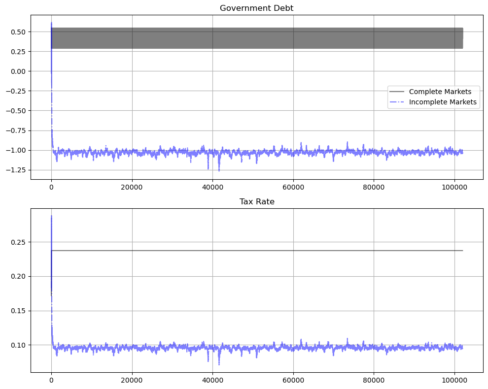
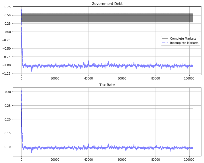
The long simulation apparently indicates eventual convergence to an ergodic distribution.

It takes about 1000 periods to reach the ergodic distribution – an outcome that is forecast by approximations to rates of convergence that appear in BEGS [Bhandari et al., 2017] and that we discuss in Fluctuating Interest Rates Deliver Fiscal Insurance.

Let’s discard the first 2000 observations of the simulation and construct the histogram of the par value of government debt.

We obtain the following graph for the histogram of the last 100,000 observations on the par value of government debt.

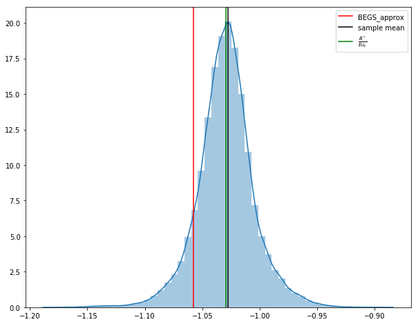
The black vertical line denotes the sample mean for the last 100,000 observations included in the histogram; the green vertical line denotes the value of \(\frac{ {\mathcal B}^*}{E u_c}\), associated with a sample from our approximation to the ergodic distribution where \({\mathcal B}^*\) is a regression coefficient to be described below; the red vertical line denotes an approximation by [Bhandari et al., 2017] to the mean of the ergodic distribution that can be computed before the ergodic distribution has been approximated, as described below.

Before moving on to discuss the histogram and the vertical lines approximating the ergodic mean of government debt in more detail, the following graphs show government debt and taxes early in the simulation, for periods 1-100 and 101 to 200 respectively.

titles = ['Government Debt', 'Tax Rate']

fig, axes = plt.subplots(4, 1, figsize=(10, 15))

for i, id in enumerate([2, 3]):
    axes[i].plot(sim_seq_long[id][:99], '-k', sim_bel_long[id][:99],
                 '-.b', alpha=0.5)
    axes[i+2].plot(range(100, 199), sim_seq_long[id][100:199], '-k',
                   range(100, 199), sim_bel_long[id][100:199], '-.b',
                   alpha=0.5)
    axes[i].set(title=titles[i])
    axes[i+2].set(title=titles[i])
    axes[i].grid()
    axes[i+2].grid()

axes[0].legend(('Complete Markets', 'Incomplete Markets'))
plt.tight_layout()
plt.show()

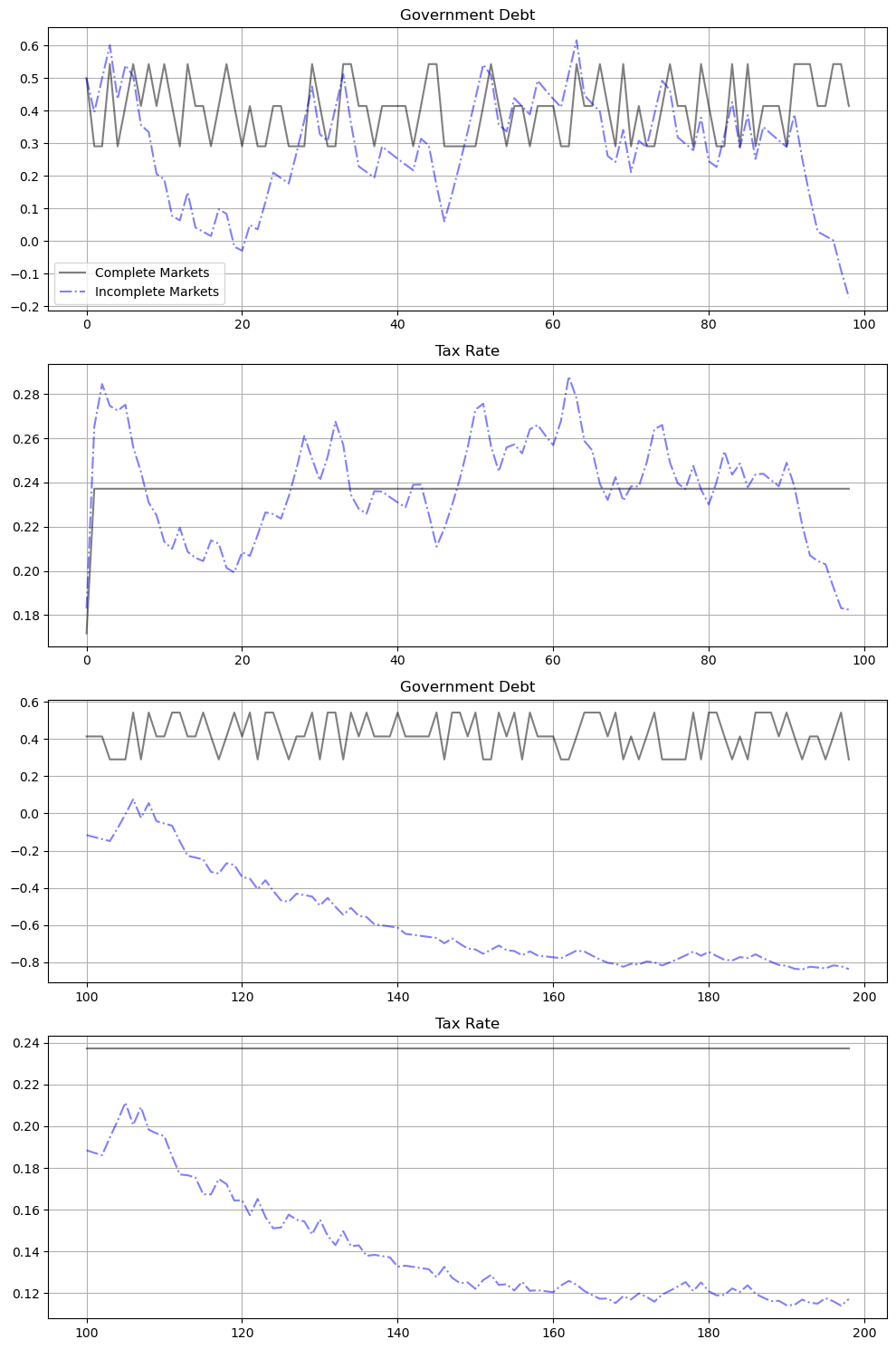
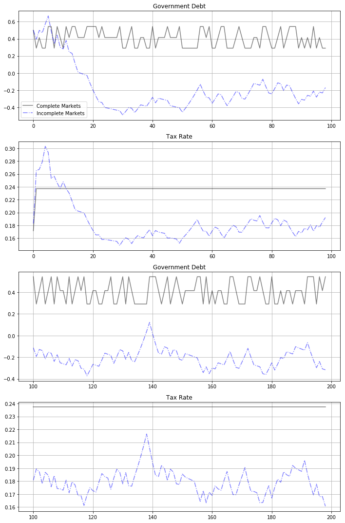
_images/ea99b7d1aa6aefee6895d3abefad68f80fdf618d5a4e4e0804712e613b340a9f.png

For the short samples early in our simulated sample of 102,000 observations, fluctuations in government debt and the tax rate conceal the weak but inexorable force that the Ramsey planner puts into both series driving them toward ergodic marginal distributions that are far from these early observations

early observations are more influenced by the initial value of the par value of government debt than by the ergodic mean of the par value of government debt
much later observations are more influenced by the ergodic mean and are independent of the par value of initial government debt

48.4. Asymptotic Mean and Rate of Convergence#

We apply the results of BEGS [Bhandari et al., 2017] to interpret

the mean of the ergodic distribution of government debt
the rate of convergence to the ergodic distribution from an arbitrary initial government debt

We begin by computing objects required by the theory of section III.i of BEGS [Bhandari et al., 2017].

As in Fiscal Insurance via Fluctuating Interest Rates, we recall that BEGS [Bhandari et al., 2017] used a particular notation to represent what we can regard as their generalization of an AMSS model.

We introduce some of the [Bhandari et al., 2017] notation so that readers can quickly relate notation that appears in key BEGS formulas to the notation that we have used in previous lectures here and here.

BEGS work with objects \(B_t, {\mathcal B}_t, {\mathcal R}_t, {\mathcal X}_t\) that are related to notation that we used in earlier lectures by

\[\begin{split} \begin{aligned} {\mathcal R}_t & = \frac{u_{c,t}}{u_{c,t-1}} R_{t-1} = \frac{u_{c,t}}{ \beta E_{t-1} u_{c,t}} \\ B_t & = \frac{b_{t+1}(s^t)}{R_t(s^t)} \\ b_t(s^{t-1}) & = {\mathcal R}_{t-1} B_{t-1} \\ {\mathcal B}_t & = u_{c,t} B_t = (\beta E_t u_{c,t+1}) b_{t+1}(s^t) \\ {\mathcal X}_t & = u_{c,t} [g_t - \tau_t n_t] \end{aligned} \end{split}\]

BEGS [Bhandari et al., 2017] call \({\mathcal X}_t\) the effective government deficit and \({\mathcal B}_t\) the effective government debt.

Equation (44) of [Bhandari et al., 2017] expresses the time \(t\) state \(s\) government budget constraint as

(48.1)#\[{\mathcal B}(s) = {\mathcal R}_\tau(s, s_{-}) {\mathcal B}_{-} + {\mathcal X}_{\tau} (s)\]

where the dependence on \(\tau\) is meant to remind us that these objects depend on the tax rate; \(s_{-}\) is last period’s Markov state.

BEGS interpret random variations in the right side of (48.1) as fiscal risks generated by

interest-rate-driven fluctuations in time \(t\) effective payments due on the government portfolio, namely, \({\mathcal R}_\tau(s, s_{-}) {\mathcal B}_{-}\), and
fluctuations in the effective government deficit \({\mathcal X}_t\)

48.4.1. Asymptotic Mean#

BEGS give conditions under which the ergodic mean of \({\mathcal B}_t\) is approximated by

(48.2)#\[{\mathcal B}^* = - \frac{\rm cov^{\infty}({\mathcal R}_t, {\mathcal X_t})}{\rm var^{\infty}({\mathcal R}_t)}\]

where the superscript \(\infty\) denotes a moment taken with respect to an ergodic distribution.

Formula (48.2) represents \({\mathcal B}^*\) as a regression coefficient of \({\mathcal X}_t\) on \({\mathcal R}_t\) in the ergodic distribution.

Regression coefficient \({\mathcal B}^*\) solves a variance-minimization problem:

(48.3)#\[{\mathcal B}^* = {\rm argmin}_{\mathcal B} {\rm var}^\infty ({\mathcal R} {\mathcal B} + {\mathcal X})\]

The minimand in criterion (48.3) measures fiscal risk associated with a given tax-debt policy that appears on the right side of equation (48.1).

Expressing formula (48.2) in terms of our notation tells us that the ergodic mean of the par value \(b\) of government debt in the AMSS model should be approximately

(48.4)#\[\hat b = \frac{\mathcal B^*}{\beta E( E_t u_{c,t+1})} = \frac{\mathcal B^*}{\beta E( u_{c,t+1} )}\]

where mathematical expectations are taken with respect to the ergodic distribution.

48.4.2. Rate of Convergence#

BEGS also derive the following approximation to the rate of convergence to \({\mathcal B}^{*}\) from an arbitrary initial condition.

(48.5)#\[\frac{ E_t ( {\mathcal B}_{t+1} - {\mathcal B}^{*} )} { ( {\mathcal B}_{t} - {\mathcal B}^{*} )} \approx \frac{1}{1 + \beta^2 {\rm var}^\infty ({\mathcal R} )}\]

(See the equation above equation (47) in BEGS [Bhandari et al., 2017])

48.4.3. More Advanced Topic#

The remainder of this lecture is about technical material based on formulas from BEGS [Bhandari et al., 2017].

The topic involves interpreting and extending formula (48.3) for the ergodic mean \({\mathcal B}^*\).

48.4.4. Chicken and Egg#

Notice how attributes of the ergodic distribution for \({\mathcal B}_t\) appear on the right side of formula (48.3) for approximating the ergodic mean via \({\mathcal B}^*\).

Therefor, formula (48.3) is not useful for estimating the mean of the ergodic in advance of actually approximating the ergodic distribution.

we need to know the ergodic distribution to compute the right side of formula (48.3)

So the primary use of equation (48.3) is how it confirms that the ergodic distribution solves a fiscal-risk minimization problem.

As an example, notice how we used the formula for the mean of \({\mathcal B}\) in the ergodic distribution of the special AMSS economy in Fiscal Insurance via Fluctuating Interest Rates

first we computed the ergodic distribution using a reverse-engineering construction
then we verified that \({\mathcal B}^*\) agrees with the mean of that distribution

48.4.5. Approximating the Ergodic Mean#

BEGS also [Bhandari et al., 2017] propose an approximation to \({\mathcal B}^*\) that can be computed without first approximating the ergodic distribution.

To construct the BEGS approximation to \({\mathcal B}^*\), we just follow steps set forth on pages 648 - 650 of section III.D of [Bhandari et al., 2017]

notation in BEGS might be confusing at first sight, so it is important to stare and digest before computing
there are also some sign errors in the [Bhandari et al., 2017] text that we’ll want to correct here

Here is a step-by-step description of the BEGS [Bhandari et al., 2017] approximation procedure.

48.4.6. Step by Step#

Step 1: For a given \(\tau\) we compute a vector of values \(c_\tau(s), s= 1, 2, \ldots, S\) that satisfy

\[ (1-\tau) c_\tau(s)^{-\sigma} - (c_{\tau}(s) + g(s))^{\gamma} = 0 \]

This is a nonlinear equation to be solved for \(c_{\tau}(s), s = 1, \ldots, S\).

\(S=3\) in our case, but we’ll write code for a general integer \(S\).

Typo alert: Please note that there is a sign error in equation (42) of BEGS [Bhandari et al., 2017] – it should be a minus rather than a plus in the middle.

We have made the appropriate correction in the above equation.

Step 2: Knowing \(c_\tau(s), s=1, \ldots, S\) for a given \(\tau\), we want to compute the random variables

\[ {\mathcal R}_\tau(s) = \frac{c_\tau(s)^{-\sigma}}{\beta \sum_{s'=1}^S c_\tau(s')^{-\sigma} \pi(s')} \]

and

\[ {\mathcal X}_\tau(s) = (c_\tau(s) + g(s))^{1+ \gamma} - c_\tau(s)^{1-\sigma} \]

each for \(s= 1, \ldots, S\).

BEGS call \({\mathcal R}_\tau(s)\) the effective return on risk-free debt and they call \({\mathcal X}_\tau(s)\) the effective government deficit.

Step 3: With the preceding objects in hand, for a given \({\mathcal B}\), we seek a \(\tau\) that satisfies

\[ {\mathcal B} = - \frac{\beta} {1-\beta} E {\mathcal X_\tau} \equiv - \frac{\beta} {1-\beta} \sum_{s} {\mathcal X}_\tau(s) \pi(s) \]

This equation says that at a constant discount factor \(\beta\), equivalent government debt \({\mathcal B}\) equals the present value of the mean effective government surplus.

Another typo alert: there is a sign error in equation (46) of BEGS [Bhandari et al., 2017] –the left side should be multiplied by \(-1\).

We have made this correction in the above equation.

For a given \({\mathcal B}\), let a \(\tau\) that solves the above equation be called \(\tau(\mathcal B)\).

We’ll use a Python root solver to find a \(\tau\) that solves this equation for a given \({\mathcal B}\).

We’ll use this function to induce a function \(\tau({\mathcal B})\).

Step 4: With a Python program that computes \(\tau(\mathcal B)\) in hand, next we write a Python function to compute the random variable.

\[ J({\mathcal B})(s) = \mathcal R_{\tau({\mathcal B})}(s) {\mathcal B} + {\mathcal X}_{\tau({\mathcal B})}(s) , \quad s = 1, \ldots, S \]

Step 5: Now that we have a way to compute the random variable \(J({\mathcal B})(s), s= 1, \ldots, S\), via a composition of Python functions, we can use the population variance function that we defined in the code above to construct a function \({\rm var}(J({\mathcal B}))\).

We put \({\rm var}(J({\mathcal B}))\) into a Python function minimizer and compute

\[ {\mathcal B}^* = {\rm argmin}_{\mathcal B} {\rm var } (J({\mathcal B}) ) \]

Step 6: Next we take the minimizer \({\mathcal B}^*\) and the Python functions for computing means and variances and compute

\[ {\rm rate} = \frac{1}{1 + \beta^2 {\rm var}( {\mathcal R}_{\tau({\mathcal B}^*)} )} \]

Ultimate outputs of this string of calculations are two scalars

\[ ({\mathcal B}^*, {\rm rate} ) \]

Step 7: Compute the divisor

\[ div = {\beta E u_{c,t+1}} \]

and then compute the mean of the par value of government debt in the AMSS model

\[ \hat b = \frac{ {\mathcal B}^*}{div} \]

In the two-Markov-state AMSS economy in Fiscal Insurance via Fluctuating Interest Rates, \(E_t u_{c,t+1} = E u_{c,t+1}\) in the ergodic distribution.

We have confirmed that this formula very accurately describes a constant par value of government debt that

supports full fiscal insurance via fluctuating interest parameters, and
is the limit of government debt as \(t \rightarrow +\infty\)

In the three-Markov-state economy of this lecture, the par value of government debt fluctuates in a history-dependent way even asymptotically.

In this economy, \(\hat b\) given by the above formula approximates the mean of the ergodic distribution of the par value of government debt

so while the approximation circumvents the chicken and egg problem that surrounds: the much better approximation associated with the green vertical line, it does so by enlarging the approximation error

\(\hat b\) is represented by the red vertical line plotted in the histogram of the last 100,000 observations of our simulation of the par value of government debt plotted above
the approximation is fairly accurate but not perfect

48.4.7. Execution#

Now let’s move on to compute things step by step.

48.4.7.1. Step 1#

u = CRRAutility(π=np.full((3, 3), 1 / 3),
                G=np.array([0.1, 0.2, .3]),
                Θ=np.ones(3))

τ = 0.05           # Initial guess of τ (to displays calcs along the way)
S = len(u.G)       # Number of states

def solve_c(c, τ, u):
    return (1 - τ) * c**(-u.σ) - (c + u.G)**u.γ

# .x returns the result from root
c = root(solve_c, np.ones(S), args=(τ, u)).x
c

array([0.93852387, 0.89231015, 0.84858872])

root(solve_c, np.ones(S), args=(τ, u))

 message: The solution converged.
 success: True
  status: 1
     fun: [ 5.618e-10 -4.769e-10  1.175e-11]
       x: [ 9.385e-01  8.923e-01  8.486e-01]
  method: hybr
    nfev: 11
    fjac: [[-9.999e-01 -4.954e-03 -1.261e-02]
           [-5.156e-03  9.999e-01  1.610e-02]
           [-1.253e-02 -1.616e-02  9.998e-01]]
       r: [ 4.269e+00  8.685e-02 -6.301e-02 -4.713e+00 -7.433e-02
           -5.508e+00]
     qtf: [ 1.556e-08  1.283e-08  7.899e-11]

48.4.7.2. Step 2#

n = c + u.G   # Compute labor supply

48.4.8. Note about Code#

Remember that in our code \(\pi\) is a \(3 \times 3\) transition matrix.

But because we are studying an IID case, \(\pi\) has identical rows and we need only to compute objects for one row of \(\pi\).

This explains why at some places below we set \(s=0\) just to pick off the first row of \(\pi\).

48.4.9. Running the code#

Let’s take the code out for a spin.

First, let’s compute \({\mathcal R}\) and \({\mathcal X}\) according to our formulas

def compute_R_X(τ, u, s):
    c = root(solve_c, np.ones(S), args=(τ, u)).x  # Solve for vector of c's
    div = u.β * (u.Uc(c[0], n[0]) * u.π[s, 0]  \
                 +  u.Uc(c[1], n[1]) * u.π[s, 1] \
                 +  u.Uc(c[2], n[2]) * u.π[s, 2])
    R = c**(-u.σ) / (div)
    X = (c + u.G)**(1 + u.γ) - c**(1 - u.σ)
    return R, X

c**(-u.σ) @ u.π

array([1.25997521, 1.25997521, 1.25997521])

u.π

array([[0.33333333, 0.33333333, 0.33333333],
       [0.33333333, 0.33333333, 0.33333333],
       [0.33333333, 0.33333333, 0.33333333]])

We only want unconditional expectations because we are in an IID case.

So we’ll set \(s=0\) and just pick off expectations associated with the first row of \(\pi\)

s = 0

R, X = compute_R_X(τ, u, s)

Let’s look at the random variables \({\mathcal R}, {\mathcal X}\)

array([1.00116313, 1.10755123, 1.22461897])

mean(R, s)

1.1111111111111112

array([0.05457803, 0.18259396, 0.33685546])

mean(X, s)

0.19134248445303795

X @ u.π

array([0.19134248, 0.19134248, 0.19134248])

48.4.9.1. Step 3#

def solve_τ(τ, B, u, s):
    R, X = compute_R_X(τ, u, s)
    return ((u.β - 1) / u.β) * B - X @ u.π[s]

Note that \(B\) is a scalar.

Let’s try out our method computing \(\tau\)

s = 0
B = 1.0

τ = root(solve_τ, .1, args=(B, u, s)).x[0]  # Very sensitive to initial value
τ

0.2740159773695818

In the above cell, B is fixed at 1 and \(\tau\) is to be computed as a function of B.

Note that 0.2 is the initial value for \(\tau\) in the root-finding algorithm.

48.4.9.2. Step 4#

def min_J(B, u, s):
    # Very sensitive to initial value of τ
    τ = root(solve_τ, .5, args=(B, u, s)).x[0]
    R, X = compute_R_X(τ, u, s)
    return variance(R * B + X, s)

min_J(B, u, s)

0.035564405653720765

48.4.9.3. Step 6#

B_star = minimize(min_J, .5, args=(u, s)).x[0]
B_star

-1.199483167941158

n = c + u.G  # Compute labor supply

div = u.β * (u.Uc(c[0], n[0]) * u.π[s, 0]  \
             +  u.Uc(c[1], n[1]) * u.π[s, 1] \
             +  u.Uc(c[2], n[2]) * u.π[s, 2])

B_hat = B_star/div
B_hat

-1.0577661126390971

τ_star = root(solve_τ, 0.05, args=(B_star, u, s)).x[0]
τ_star

0.09572916798461703

R_star, X_star = compute_R_X(τ_star, u, s)
R_star, X_star

(array([0.9998398 , 1.10746593, 1.2260276 ]),
 array([0.0020272 , 0.12464752, 0.27315299]))

rate = 1 / (1 + u.β**2 * variance(R_star, s))
rate

0.9931353432732218

root(solve_c, np.ones(S), args=(τ_star, u)).x

array([0.9264382 , 0.88027117, 0.83662635])