18. Lucas Asset Pricing Using DLE #

Contents

Lucas Asset Pricing Using DLE
- Asset Pricing Equations
- Asset Pricing Simulations

This is one of a suite of lectures that use the quantecon DLE class to instantiate models within the [HS13] class of models described in detail in Recursive Models of Dynamic Linear Economies.

In addition to what’s in Anaconda, this lecture uses the quantecon library

!pip install --upgrade quantecon

This lecture uses the DLE class to price payout streams that are linear functions of the economy’s state vector, as well as risk-free assets that pay out one unit of the first consumption good with certainty.

We assume basic knowledge of the class of economic environments that fall within the domain of the DLE class.

Many details about the basic environment are contained in the lecture Growth in Dynamic Linear Economies.

We’ll also need the following imports

import numpy as np
import matplotlib.pyplot as plt
from quantecon import DLE
%matplotlib inline

We use a linear-quadratic version of an economy that Lucas (1978) [Luc78] used to develop an equilibrium theory of asset prices:

Preferences

\[ -\frac{1}{2}\mathbb{E}\sum_{t=0}^\infty \beta^t[(c_t - b_t)^2 + l_t^2]|J_0 \]

\[ s_t = c_t \]

\[ b_t = U_bz_t \]

Technology

\[ c_t = d_{1t} \]

\[ k_t = \delta_k k_{t-1} + i_t \]

\[ g_t = \phi_1 i_t \, , \phi_1 > 0 \]

\[\begin{split} \left[ {\begin{array}{c} d_{1t} \\ 0 \end{array} } \right] = U_dz_t \end{split}\]

Information

\[\begin{split} z_{t+1} = \left[ {\begin{array}{ccc} 1 & 0 & 0 \\ 0 & 0.8 & 0 \\ 0 & 0 & 0.5 \end{array} } \right] z_t + \left[ {\begin{array}{cc} 0 & 0 \\ 1 & 0 \\ 0 & 1 \end{array} } \right] w_{t+1} \end{split}\]

\[ U_b = \left[ {\begin{array}{ccc} 30 & 0 & 0 \end{array} } \right] \]

\[\begin{split} U_d = \left[ {\begin{array}{ccc} 5 & 1 & 0 \\ 0 & 0 & 0 \end{array} } \right] \end{split}\]

\[ x_0 = \left[ {\begin{array}{ccccc} 5 & 150 & 1 & 0 & 0 \end{array} } \right]' \]

18.1. Asset Pricing Equations #

[HS13] show that the time t value of a permanent claim to a stream \(y_s = U_ax_s \, , s \geq t\) is:

\[ a_t = (x_t'\mu_ax_t + \sigma_a)/(\bar e _1M_cx_t) \]

with

\[ \mu_a = \sum_{\tau = 0}^\infty \beta^\tau(A^{o'})^\tau Z_a A^{o\tau} \]

\[ \sigma_a = \frac{\beta}{1-\beta} \text{trace} (Z_a \sum_{\tau = 0}^\infty \beta^\tau (A^{o})^\tau C C^{'} (A^{o'})^\tau) \]

where

\[ Z_a = U_a^{'}M_c \]

The use of \(\bar e _1\) indicates that the first consumption good is the numeraire.

18.2. Asset Pricing Simulations #

gam = 0
γ = np.array([[gam], [0]])
ϕ_c = np.array([[1], [0]])
ϕ_g = np.array([[0], [1]])
ϕ_1 = 1e-4
ϕ_i = np.array([[0], [-ϕ_1]])
δ_k = np.array([[.95]])
θ_k = np.array([[1]])
β = np.array([[1 / 1.05]])
ud = np.array([[5, 1, 0],
               [0, 0, 0]])
a22 = np.array([[1,   0,    0],
                [0, 0.8,    0],
                [0,   0, 0.5]])
c2 = np.array([[0, 1, 0],
               [0, 0, 1]]).T
l_λ = np.array([[0]])
π_h = np.array([[1]])
δ_h = np.array([[.9]])
θ_h = np.array([[1]]) - δ_h
ub = np.array([[30, 0, 0]])
x0 = np.array([[5, 150, 1, 0, 0]]).T

info1 = (a22, c2, ub, ud)
tech1 = (ϕ_c, ϕ_g, ϕ_i, γ, δ_k, θ_k)
pref1 = (β, l_λ, π_h, δ_h, θ_h)

econ1 = DLE(info1, tech1, pref1)

After specifying a “Pay” matrix, we simulate the economy.

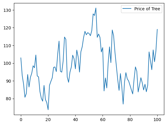
The particular choice of “Pay” used below means that we are pricing a perpetual claim on the endowment process \(d_{1t}\)

econ1.compute_sequence(x0, ts_length=100, Pay=np.array([econ1.Sd[0, :]]))

The graph below plots the price of this claim over time:

### Fig 7.12.1 from p.147 of HS2013
plt.plot(econ1.Pay_Price, label='Price of Tree')
plt.legend()
plt.show()

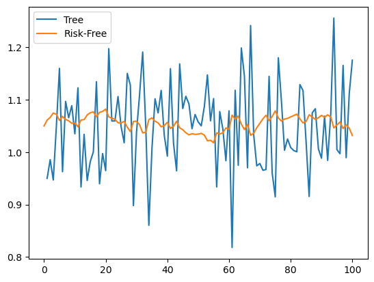
_images/002a556769e1ccef3b0ec9b0865befa965f2cc330a85db706822de6e10360e8c.png

The next plot displays the realized gross rate of return on this “Lucas tree” as well as on a risk-free one-period bond:

### Left panel of Fig 7.12.2 from p.148 of HS2013
plt.plot(econ1.Pay_Gross, label='Tree')
plt.plot(econ1.R1_Gross, label='Risk-Free')
plt.legend()
plt.show()

_images/f47bb2f13d90b48d2fd73c2ac6710dffa41bb9e889cca9d49b861e6826d28185.png

np.corrcoef(econ1.Pay_Gross[1:, 0], econ1.R1_Gross[1:, 0])

array([[ 1.        , -0.48190497],
       [-0.48190497,  1.        ]])

Above we have also calculated the correlation coefficient between these two returns.

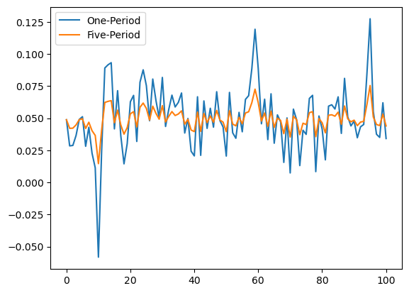
To give an idea of how the term structure of interest rates moves in this economy, the next plot displays the net rates of return on one-period and five-period risk-free bonds:

### Right panel of Fig 7.12.2 from p.148 of HS2013
plt.plot(econ1.R1_Net, label='One-Period')
plt.plot(econ1.R5_Net, label='Five-Period')
plt.legend()
plt.show()

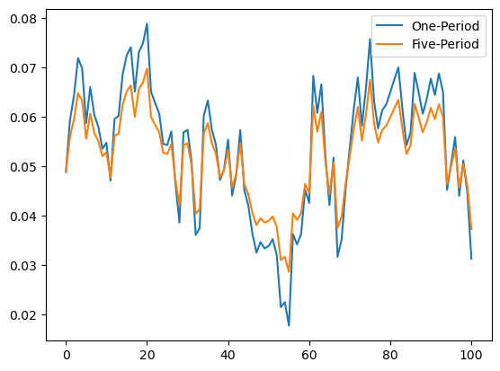
_images/668c65bd76824adf3beb707a29d6212cecfc8f3f4c3e381ea65424db55548956.png

From the above plot, we can see the tendency of the term structure to slope up when rates are low and to slope down when rates are high.

Comparing it to the previous plot of the price of the “Lucas tree”, we can also see that net rates of return are low when the price of the tree is high, and vice versa.

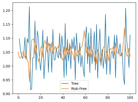
We now plot the realized gross rate of return on a “Lucas tree” as well as on a risk-free one-period bond when the autoregressive parameter for the endowment process is reduced to 0.4:

a22_2 = np.array([[1,   0,   0],
                  [0, 0.4,   0],
                  [0,   0, 0.5]])
info2 = (a22_2, c2, ub, ud)

econ2 = DLE(info2, tech1, pref1)
econ2.compute_sequence(x0, ts_length=100, Pay=np.array([econ2.Sd[0, :]]))

### Left panel of Fig 7.12.3 from p.148 of HS2013
plt.plot(econ2.Pay_Gross, label='Tree')
plt.plot(econ2.R1_Gross, label='Risk-Free')
plt.legend()
plt.show()

_images/e6435d462607f663e31a74a98a3ceb6cb2a8c9ae6212f15038f8e04a44c68ded.png

np.corrcoef(econ2.Pay_Gross[1:, 0], econ2.R1_Gross[1:, 0])

array([[ 1.       , -0.6777561],
       [-0.6777561,  1.       ]])

The correlation between these two gross rates is now more negative.

Next, we again plot the net rates of return on one-period and five-period risk-free bonds:

### Right panel of Fig 7.12.3 from p.148 of HS2013
plt.plot(econ2.R1_Net, label='One-Period')
plt.plot(econ2.R5_Net, label='Five-Period')
plt.legend()
plt.show()

_images/b63b45864c8f2b5d3c62b4329a8a12d31842ae381458db573baeb9b83fc9eb5a.png

We can see the tendency of the term structure to slope up when rates are low (and down when rates are high) has been accentuated relative to the first instance of our economy.

18. Lucas Asset Pricing Using DLE#

18.1. Asset Pricing Equations#

18.2. Asset Pricing Simulations#

18. Lucas Asset Pricing Using DLE #

18.1. Asset Pricing Equations #

18.2. Asset Pricing Simulations #