55. Optimal Taxation without State-Contingent Debt#
55.1. Overview#
In another lecture, we presented a special case of a model of optimal taxation with state-contingent debt due to Robert E. Lucas, Jr., and Nancy Stokey [Lucas and Stokey, 1983].
In this lecture, we describe how Aiyagari, Marcet, Sargent, and Seppälä [Aiyagari et al., 2002] (hereafter, AMSS) modified that model.
In a nutshell, AMSS studied optimal taxation in a version of Lucas and Stokey’s environment without state-contingent debt.
In this lecture, we
describe AMSS’s assumptions and equilibrium concept
describe how to solve the model using a different approach than AMSS did
implement the model numerically
conduct some policy experiments
compare outcomes with those in a corresponding complete-markets model
In addition to what’s in Anaconda, this lecture will need the following libraries:
!pip install --upgrade quantecon
Let’s start with following imports:
import numpy as np
import matplotlib.pyplot as plt
from scipy.optimize import root
from quantecon import optimize, MarkovChain
from numba import njit, prange, float64
from numba.experimental import jitclass
Now let’s define numba-compatible interpolation functions for this lecture.
We will soon use the following interpolation functions to interpolate the value function and the policy functions
@njit
def get_grid_nodes(grid):
    """
    Get the actual grid points from a grid tuple.
    """
    x_min, x_max, x_num = grid
    return np.linspace(x_min, x_max, x_num)

@njit
def linear_interp_1d_scalar(x_min, x_max, x_num, y_values, x_val):
    """Helper function for scalar interpolation"""
    x_nodes = np.linspace(x_min, x_max, x_num)

    # Extrapolation with linear extension
    if x_val <= x_nodes[0]:
        # Linear extrapolation using first two points
        if x_num >= 2:
            slope = (y_values[1] - y_values[0]) \
              / (x_nodes[1] - x_nodes[0])
            return y_values[0] + slope * (x_val - x_nodes[0])
        else:
            return y_values[0]

    if x_val >= x_nodes[-1]:
        # Linear extrapolation using last two points
        if x_num >= 2:
            slope = (y_values[-1] - y_values[-2]) \
              / (x_nodes[-1] - x_nodes[-2])
            return y_values[-1] + slope * (x_val - x_nodes[-1])
        else:
            return y_values[-1]

    # Binary search for the right interval
    left = 0
    right = x_num - 1
    while right - left > 1:
        mid = (left + right) // 2
        if x_nodes[mid] <= x_val:
            left = mid
        else:
            right = mid

    # Linear interpolation
    x_left = x_nodes[left]
    x_right = x_nodes[right]
    y_left = y_values[left]
    y_right = y_values[right]

    weight = (x_val - x_left) / (x_right - x_left)
    return y_left * (1 - weight) + y_right * weight

@njit
def linear_interp_1d(x_grid, y_values, x_query):
    """
    Perform 1D linear interpolation.
    """
    x_min, x_max, x_num = x_grid
    return linear_interp_1d_scalar(x_min, x_max, x_num, y_values, x_query[0])
We begin with an introduction to the model.
55.2. Competitive equilibrium with distorting taxes#
Many but not all features of AMSS’s economy are identical to those of the Lucas-Stokey economy.
Let’s start with things that are identical.
For \(t \geq 0\), a history of the state is represented by \(s^t = [s_t, s_{t-1}, \ldots, s_0]\).
Government purchases \(g(s)\) are an exact time-invariant function of \(s\).
Let \(c_t(s^t)\), \(\ell_t(s^t)\), and \(n_t(s^t)\) denote consumption, leisure, and labor supply, respectively, at history \(s^t\) at time \(t\).
Each period a representative household is endowed with one unit of time that can be divided between leisure \(\ell_t\) and labor \(n_t\):
Output equals \(n_t(s^t)\) and can be divided between consumption \(c_t(s^t)\) and \(g(s_t)\)
Output is not storable.
The technology pins down a pre-tax wage rate to unity for all \(t, s^t\).
A representative household’s preferences over \(\{c_t(s^t), \ell_t(s^t)\}_{t=0}^\infty\) are ordered by
where
\(\pi_t(s^t)\) is a joint probability distribution over the sequence \(s^t\), and
the utility function \(u\) is increasing, strictly concave, and three times continuously differentiable in both arguments.
The government imposes a flat rate tax \(\tau_t(s^t)\) on labor income at time \(t\), history \(s^t\).
Lucas and Stokey assumed that there are complete markets in one-period Arrow securities; also see smoothing models.
It is at this point that AMSS [Aiyagari et al., 2002] modify the Lucas and Stokey economy.
AMSS allow the government to issue only one-period risk-free debt each period.
Ruling out complete markets in this way is a step in the direction of making total tax collections behave more like that prescribed in Robert Barro (1979) [Barro, 1979] than they do in Lucas and Stokey (1983) [Lucas and Stokey, 1983].
55.2.1. Risk-free one-period debt only#
In period \(t\) and history \(s^t\), let
\(b_{t+1}(s^t)\) be the amount of the time \(t+1\) consumption good that at time \(t\), history \(s^t\) the government promised to pay
\(R_t(s^t)\) be the gross interest rate on risk-free one-period debt between periods \(t\) and \(t+1\)
\(T_t(s^t)\) be a non-negative lump-sum transfer to the representative household [1]
That \(b_{t+1}(s^t)\) is the same for all realizations of \(s_{t+1}\) captures its risk-free character.
The market value at time \(t\) of government debt maturing at time \(t+1\) equals \(b_{t+1}(s^t)\) divided by \(R_t(s^t)\).
The government’s budget constraint in period \(t\) at history \(s^t\) is
where \(z_t(s^t)\) is the net-of-interest government surplus.
To rule out Ponzi schemes, we assume that the government is subject to a natural debt limit (to be discussed in a forthcoming lecture).
The consumption Euler equation for a representative household able to trade only one-period risk-free debt with one-period gross interest rate \(R_t(s^t)\) is
Substituting this expression into the government’s budget constraint (55.4) yields:
Components of \(z_t(s^t)\) on the right side depend on \(s^t\), but the left side is required to depend only on \(s^{t-1}\) .
This is what it means for one-period government debt to be risk-free.
Therefore, the right side of equation (55.5) also has to depend only on \(s^{t-1}\).
This requirement will give rise to measurability constraints on the Ramsey allocation to be discussed soon.
If we replace \(b_{t+1}(s^t)\) on the right side of equation (55.5) by the right side of next period’s budget constraint (associated with a particular realization \(s_{t}\)) we get
After making similar repeated substitutions for all future occurrences of government indebtedness, and by invoking a natural debt limit, we arrive at:
Notice how the conditioning sets in equation (55.6) differ: they are \(s^{t-1}\) on the left side and \(s^t\) on the right side.
Now let’s
substitute the resource constraint into the net-of-interest government surplus, and
use the household’s first-order condition \(1-\tau^n_t(s^t)= u_{\ell}(s^t) /u_c(s^t)\) to eliminate the labor tax rate
so that we can express the net-of-interest government surplus \(z_t(s^t)\) as
If we substitute appropriate versions of the right side of (55.7) for \(z_{t+j}(s^{t+j})\) into equation (55.6), we obtain a sequence of implementability constraints on a Ramsey allocation in an AMSS economy.
Expression (55.6) at time \(t=0\) and initial state \(s^0\) was also an implementability constraint on a Ramsey allocation in a Lucas-Stokey economy:
Indeed, it was the only implementability constraint there.
But now we also have a large number of additional implementability constraints
Equation (55.9) must hold for each \(s^t\) for each \(t \geq 1\).
55.2.2. Comparison with Lucas-Stokey economy#
The expression on the right side of (55.9) in the Lucas-Stokey (1983) economy would equal the present value of a continuation stream of government net-of-interest surpluses evaluated at what would be competitive equilibrium Arrow-Debreu prices at date \(t\).
In the Lucas-Stokey economy, that present value is measurable with respect to \(s^t\).
In the AMSS economy, the restriction that government debt be risk-free imposes that that same present value must be measurable with respect to \(s^{t-1}\).
In a language used in the literature on incomplete markets models, it can be said that the AMSS model requires that at each \((t, s^t)\) what would be the present value of continuation government net-of-interest surpluses in the Lucas-Stokey model must belong to the marketable subspace of the AMSS model.
55.2.3. Ramsey problem without state-contingent debt#
After we have substituted the resource constraint into the utility function, we can express the Ramsey problem as being to choose an allocation that solves
where the maximization is subject to
and
given \(b_0(s^{-1})\).
55.2.3.1. Lagrangian formulation#
Let \(\gamma_0(s^0)\) be a non-negative Lagrange multiplier on constraint (55.10).
As in the Lucas-Stokey economy, this multiplier is strictly positive when the government must resort to distortionary taxation; otherwise it equals zero.
A consequence of the assumption that there are no markets in state-contingent securities and that a market exists only in a risk-free security is that we have to attach a stochastic process \(\{\gamma_t(s^t)\}_{t=1}^\infty\) of Lagrange multipliers to the implementability constraints (55.11).
Depending on how the constraints bind, these multipliers can be positive or negative:
A negative multiplier \(\gamma_t(s^t)<0\) means that if we could relax constraint (55.11), we would like to increase the beginning-of-period indebtedness for that particular realization of history \(s^t\).
That would let us reduce the beginning-of-period indebtedness for some other history [2].
These features flow from the fact that the government cannot use state-contingent debt and therefore cannot allocate its indebtedness efficiently across future states.
55.2.4. Some calculations#
It is helpful to apply two transformations to the Lagrangian.
Multiply constraint (55.10) by \(u_c(s^0)\) and the constraints (55.11) by \(\beta^t u_c(s^{t})\).
Then a Lagrangian for the Ramsey problem can be represented as
where
In (55.12), the second equality uses the law of iterated expectations and Abel’s summation formula (also called summation by parts, see this page).
First-order conditions with respect to \(c_t(s^t)\) can be expressed as
and with respect to \(b_t(s^t)\) as
If we substitute \(z_t(s^t)\) from (55.7) and its derivative \(z_c(s^t)\) into the first-order condition (55.14), we find two differences from the corresponding condition for the optimal allocation in a Lucas-Stokey economy with state-contingent government debt.
The term involving \(b_t(s^{t-1})\) in the first-order condition (55.14) does not appear in the corresponding expression for the Lucas-Stokey economy.
This term reflects the constraint that beginning-of-period government indebtedness must be the same across all realizations of next period’s state, a constraint that would not be present if government debt could be state-contingent.
The Lagrange multiplier \(\Psi_t(s^t)\) in the first-order condition (55.14) may change over time in response to realizations of the state, while the multiplier \(\Phi\) in the Lucas-Stokey economy is time-invariant.
We need some code from an earlier lecture on optimal taxation with state-contingent debt sequential allocation implementation:
class SequentialLS:

    '''
    Class that takes a preference object, state transition matrix,
    and state contingent government expenditure plan as inputs, and
    solves the sequential allocation problem described above.
    It returns optimal allocations about consumption and labor supply,
    as well as the multiplier on the implementability constraint Φ.
    '''

    def __init__(self,
                 pref,
                 π=np.full((2, 2), 0.5),
                 g=np.array([0.1, 0.2])):

        # Initialize from pref object attributes
        self.β, self.π, self.g = pref.β, π, g
        self.mc = MarkovChain(self.π)
        self.S = len(π)  # Number of states
        self.pref = pref

        # Find the first best allocation
        self.find_first_best()

    def FOC_first_best(self, c, g):
        '''
        First order conditions that characterize
        the first best allocation.
        '''

        pref = self.pref
        Uc, Ul = pref.Uc, pref.Ul

        n = c + g
        l = 1 - n

        return Uc(c, l) - Ul(c, l)

    def find_first_best(self):
        '''
        Find the first best allocation
        '''
        S, g = self.S, self.g

        res = root(self.FOC_first_best, np.full(S, 0.5), args=(g,))

        if (res.fun > 1e-10).any():
            raise Exception('Could not find first best')

        self.cFB = res.x
        self.nFB = self.cFB + g

    def FOC_time1(self, c, Φ, g):
        '''
        First order conditions that characterize
        optimal time 1 allocation problems.
        '''

        pref = self.pref
        Uc, Ucc, Ul, Ull, Ulc = pref.Uc, pref.Ucc, pref.Ul, pref.Ull, pref.Ulc

        n = c + g
        l = 1 - n

        LHS = (1 + Φ) * Uc(c, l) + Φ * (c * Ucc(c, l) - n * Ulc(c, l))
        RHS = (1 + Φ) * Ul(c, l) + Φ * (c * Ulc(c, l) - n * Ull(c, l))

        diff = LHS - RHS

        return diff

    def time1_allocation(self, Φ):
        '''
        Computes optimal allocation for time t >= 1 for a given Φ
        '''
        pref = self.pref
        S, g = self.S, self.g

        # use the first best allocation as intial guess
        res = root(self.FOC_time1, self.cFB, args=(Φ, g))

        if (res.fun > 1e-10).any():
            raise Exception('Could not find LS allocation.')

        c = res.x
        n = c + g
        l = 1 - n

        # Compute x
        I = pref.Uc(c, n) * c - pref.Ul(c, l) * n
        x = np.linalg.solve(np.eye(S) - self.β * self.π, I)

        return c, n, x

    def FOC_time0(self, c0, Φ, g0, b0):
        '''
        First order conditions that characterize
        time 0 allocation problem.
        '''

        pref = self.pref
        Ucc, Ulc = pref.Ucc, pref.Ulc

        n0 = c0 + g0
        l0 = 1 - n0

        diff = self.FOC_time1(c0, Φ, g0)
        diff -= Φ * (Ucc(c0, l0) - Ulc(c0, l0)) * b0

        return diff

    def implementability(self, Φ, b0, s0, cn0_arr):
        '''
        Compute the differences between the RHS and LHS
        of the implementability constraint given Φ,
        initial debt, and initial state.
        '''

        pref, π, g, β = self.pref, self.π, self.g, self.β
        Uc, Ul = pref.Uc, pref.Ul
        g0 = self.g[s0]

        c, n, x = self.time1_allocation(Φ)

        res = root(self.FOC_time0, cn0_arr[0], args=(Φ, g0, b0))
        c0 = res.x
        n0 = c0 + g0
        l0 = 1 - n0

        cn0_arr[:] = c0.item(), n0.item()

        LHS = Uc(c0, l0) * b0
        RHS = Uc(c0, l0) * c0 - Ul(c0, l0) * n0 + β * π[s0] @ x

        return RHS - LHS

    def time0_allocation(self, b0, s0):
        '''
        Finds the optimal time 0 allocation given
        initial government debt b0 and state s0
        '''

        # use the first best allocation as initial guess
        cn0_arr = np.array([self.cFB[s0], self.nFB[s0]])

        res = root(self.implementability, 0., args=(b0, s0, cn0_arr))

        if (res.fun > 1e-10).any():
            raise Exception('Could not find time 0 LS allocation.')

        Φ = res.x[0]
        c0, n0 = cn0_arr

        return Φ, c0, n0

    def τ(self, c, n):
        '''
        Computes τ given c, n
        '''
        pref = self.pref
        Uc, Ul = pref.Uc, pref.Ul

        return 1 - Ul(c, 1-n) / Uc(c, 1-n)

    def simulate(self, b0, s0, T, sHist=None):
        '''
        Simulates planners policies for T periods
        '''
        pref, π, β = self.pref, self.π, self.β
        Uc = pref.Uc

        if sHist is None:
            sHist = self.mc.simulate(T, s0)

        cHist, nHist, Bhist, τHist, ΦHist = np.empty((5, T))
        RHist = np.empty(T-1)

        # Time 0
        Φ, cHist[0], nHist[0] = self.time0_allocation(b0, s0)
        τHist[0] = self.τ(cHist[0], nHist[0])
        Bhist[0] = b0
        ΦHist[0] = Φ

        # Time 1 onward
        for t in range(1, T):
            c, n, x = self.time1_allocation(Φ)
            τ = self.τ(c, n)
            u_c = Uc(c, 1-n)
            s = sHist[t]
            Eu_c = π[sHist[t-1]] @ u_c
            cHist[t], nHist[t], Bhist[t], τHist[t] = c[s], n[s], x[s] / u_c[s], τ[s]
            RHist[t-1] = Uc(cHist[t-1], 1-nHist[t-1]) / (β * Eu_c)
            ΦHist[t] = Φ

        gHist = self.g[sHist]
        yHist = nHist

        return [cHist, nHist, Bhist, τHist, gHist, yHist, sHist, ΦHist, RHist]
To analyze the AMSS model, we find it useful to adopt a recursive formulation using techniques like those in our lectures on dynamic Stackelberg models and optimal taxation with state-contingent debt.
55.3. Recursive version of AMSS model#
We now describe a recursive formulation of the AMSS economy.
We have noted that from the point of view of the Ramsey planner, the restriction to one-period risk-free securities
leaves intact the single implementability constraint on allocations (55.8) from the Lucas-Stokey economy, but
adds measurability constraints (55.6) on functions of tails of allocations at each time and history
We now explore how these constraints alter Bellman equations for a time \(0\) Ramsey planner and for time \(t \geq 1\), history \(s^t\) continuation Ramsey planners.
55.3.1. Recasting state variables#
In the AMSS setting, the government faces a sequence of budget constraints
where \(R_t(s^t)\) is the gross risk-free rate of interest between \(t\) and \(t+1\) at history \(s^t\) and \(T_t(s^t)\) are non-negative transfers.
Throughout this lecture, we shall set transfers to zero.
Note
For some issues about the limiting behavior of debt, this is possibly an important difference from AMSS [Aiyagari et al., 2002]. AMSS restricted transfers to be non-negative.
In this case, the household faces a sequence of budget constraints
The household’s first-order conditions are \(u_{c,t} = \beta R_t \mathbb E_t u_{c,t+1}\) and \((1-\tau_t) u_{c,t} = u_{l,t}\).
Using these to eliminate \(R_t\) and \(\tau_t\) from budget constraint (55.16) gives
or
Now define
and represent the household’s budget constraint at time \(t\), history \(s^t\) as
for \(t \geq 1\).
55.3.2. Measurability constraints#
Write equation (55.18) as
The right side of equation (55.21) expresses the time \(t\) value of government debt in terms of a linear combination of terms whose individual components are measurable with respect to \(s^t\).
The sum of terms on the right side of equation (55.21) must equal \(b_t(s^{t-1})\).
That implies that it has to be measurable with respect to \(s^{t-1}\).
Equations (55.21) are the measurability constraints that the AMSS model adds to the single time \(0\) implementation constraint imposed in the Lucas and Stokey model.
55.3.3. Two Bellman equations#
Let \(\Pi(s|s_-)\) be a Markov transition matrix whose entries tell probabilities of moving from state \(s_-\) to state \(s\) in one period.
Let
\(V(x_-, s_-)\) be the continuation value of a continuation Ramsey plan at \(x_{t-1} = x_-, s_{t-1} =s_-\) for \(t \geq 1\)
\(W(b, s)\) be the value of the Ramsey plan at time \(0\) at \(b_0=b\) and \(s_0 = s\)
We distinguish between two types of planners:
For \(t \geq 1\), the value function for a continuation Ramsey planner satisfies the Bellman equation
subject to the following collection of implementability constraints, one for each \(s \in {\cal S}\):
A continuation Ramsey planner at \(t \geq 1\) takes \((x_{t-1}, s_{t-1}) = (x_-, s_-)\) as given and before \(s\) is realized chooses \((n_t(s_t), x_t(s_t)) = (n(s), x(s))\) for \(s \in {\cal S}\).
The Ramsey planner takes \((b_0, s_0)\) as given and chooses \((n_0, x_0)\).
The value function \(W(b_0, s_0)\) for the time \(t=0\) Ramsey planner satisfies the Bellman equation
where maximization is subject to
55.3.4. Martingale supercedes state-variable degeneracy#
Let \(\mu(s|s_-) \Pi(s|s_-)\) be a Lagrange multiplier on the constraint (55.23) for state \(s\).
After forming an appropriate Lagrangian, we find that the continuation Ramsey planner’s first-order condition with respect to \(x(s)\) is
Applying an envelope theorem to Bellman equation (55.22) gives
Equations (55.26) and (55.27) imply that
Equation (55.28) states that \(V_x(x, s)\) is a risk-adjusted martingale.
Saying that \(V_x(x, s)\) is a risk-adjusted martingale means that \(V_x(x, s)\) is a martingale with respect to the probability distribution over \(s^t\) sequences that are generated by the twisted transition probability matrix:
Exercise 55.1
Please verify that \(\check \Pi(s|s_-)\) is a valid Markov transition density, i.e., that its elements are all non-negative and that for each \(s_-\), the sum over \(s\) equals unity.
55.3.5. Absence of state variable degeneracy#
Along a Ramsey plan, the state variable \(x_t = x_t(s^t, b_0)\) becomes a function of the history \(s^t\) and initial government debt \(b_0\).
In Lucas-Stokey model, we found that
a counterpart to \(V_x(x,s)\) is time-invariant and equal to the Lagrange multiplier on the Lucas-Stokey implementability constraint
time invariance of \(V_x(x,s)\) is the source of a key feature of the Lucas-Stokey model, namely, state variable degeneracy in which \(x_t\) is an exact time-invariant function of \(s_t\).
That \(V_x(x,s)\) varies over time according to a twisted martingale means that there is no state-variable degeneracy in the AMSS model.
In the AMSS model, both \(x\) and \(s\) are needed to describe the state.
This property of the AMSS model transmits a twisted martingale component to consumption, employment, and the tax rate.
55.3.6. Digression on non-negative transfers#
Throughout this lecture, we have imposed that transfers \(T_t = 0\).
AMSS [Aiyagari et al., 2002] instead imposed a nonnegativity constraint \(T_t\geq 0\) on transfers.
They also considered a special case of quasi-linear preferences, \(u(c,l)= c + H(l)\).
In this case, \(V_x(x,s)\leq 0\) is a non-positive martingale.
By the martingale convergence theorem \(V_x(x,s)\) converges almost surely.
Furthermore, when the Markov chain \(\Pi(s| s_-)\) and the government expenditure function \(g(s)\) are such that \(g_t\) is perpetually random, \(V_x(x, s)\) almost surely converges to zero.
For quasi-linear preferences, the first-order condition for maximizing (55.22) subject to (55.23) with respect to \(n(s)\) becomes
When \(\mu(s|s_-) = \beta V_x(x(s),x)\) converges to zero, in the limit \(u_l(s)= 1 =u_c(s)\), so that \(\tau(x(s),s) =0\).
Thus, in the limit, if \(g_t\) is perpetually random, the government accumulates sufficient assets to finance all expenditures from earnings on those assets, returning any excess revenues to the household as non-negative lump-sum transfers.
55.3.7. Code#
The recursive formulation is implemented as follows
import numpy as np
from numba import njit, prange
from quantecon import optimize

@njit
def get_grid_nodes(grid):
    """
    Get the actual grid points from a grid tuple.
    """
    x_min, x_max, x_num = grid
    return np.linspace(x_min, x_max, x_num)

@njit
def linear_interp_1d_scalar(x_min, x_max, x_num, y_values, x_val):
    """Helper function for scalar interpolation"""
    x_nodes = np.linspace(x_min, x_max, x_num)

    # Extrapolation with linear extension
    if x_val <= x_nodes[0]:
        # Linear extrapolation using first two points
        if x_num >= 2:
            slope = (y_values[1] - y_values[0]) / (x_nodes[1] - x_nodes[0])
            return y_values[0] + slope * (x_val - x_nodes[0])
        else:
            return y_values[0]

    if x_val >= x_nodes[-1]:
        # Linear extrapolation using last two points
        if x_num >= 2:
            slope = (y_values[-1] - y_values[-2]) / (x_nodes[-1] - x_nodes[-2])
            return y_values[-1] + slope * (x_val - x_nodes[-1])
        else:
            return y_values[-1]

    # Binary search for the right interval
    left = 0
    right = x_num - 1
    while right - left > 1:
        mid = (left + right) // 2
        if x_nodes[mid] <= x_val:
            left = mid
        else:
            right = mid

    # Linear interpolation
    x_left = x_nodes[left]
    x_right = x_nodes[right]
    y_left = y_values[left]
    y_right = y_values[right]

    weight = (x_val - x_left) / (x_right - x_left)
    return y_left * (1 - weight) + y_right * weight

@njit
def linear_interp_1d(x_grid, y_values, x_query):
    """
    Perform 1D linear interpolation.
    """
    x_min, x_max, x_num = x_grid
    return linear_interp_1d_scalar(x_min, x_max, x_num, y_values, x_query[0])

class AMSS:
    # WARNING: THE CODE IS EXTREMELY SENSITIVE TO CHOCIES OF PARAMETERS.
    # DO NOT CHANGE THE PARAMETERS AND EXPECT IT TO WORK

    def __init__(self, pref, β, Π, g, x_grid, bounds_v):
        self.β, self.Π, self.g = β, Π, g
        self.x_grid = x_grid
        self.n = x_grid[0][2]
        self.S = len(Π)
        self.bounds = bounds_v
        self.pref = pref

        self.T_v, self.T_w = bellman_operator_factory(Π, β, x_grid, g,
                                                      bounds_v)

        self.V_solved = False
        self.W_solved = False

    def compute_V(self, V, σ_v_star, tol_vfi, maxitr, print_itr):

        T_v = self.T_v

        self.success = False

        V_new = np.zeros_like(V)

        Δ = 1.0
        for itr in range(maxitr):
            T_v(V, V_new, σ_v_star, self.pref)

            Δ = np.max(np.abs(V_new - V))

            if Δ < tol_vfi:
                self.V_solved = True
                print('Successfully completed VFI after %i iterations'
                      % (itr+1))
                break

            if (itr + 1) % print_itr == 0:
                print('Error at iteration %i : ' % (itr + 1), Δ)

            V[:] = V_new[:]

        self.V = V
        self.σ_v_star = σ_v_star

        return V, σ_v_star

    def compute_W(self, b_0, W, σ_w_star):
        T_w = self.T_w
        V = self.V

        T_w(W, σ_w_star, V, b_0, self.pref)

        self.W = W
        self.σ_w_star = σ_w_star
        self.W_solved = True
        print('Succesfully solved the time 0 problem.')

        return W, σ_w_star

    def solve(self, V, σ_v_star,  b_0, W, σ_w_star, tol_vfi=1e-7,
              maxitr=1000, print_itr=10):
        print("===============")
        print("Solve time 1 problem")
        print("===============")
        self.compute_V(V, σ_v_star, tol_vfi, maxitr, print_itr)
        print("===============")
        print("Solve time 0 problem")
        print("===============")
        self.compute_W(b_0, W, σ_w_star)

    def simulate(self, s_hist, b_0):
        if not (self.V_solved and self.W_solved):
            msg = "V and W need to be successfully computed before simulation."
            raise ValueError(msg)

        pref = self.pref
        x_grid, g, β, S = self.x_grid, self.g, self.β, self.S
        σ_v_star, σ_w_star = self.σ_v_star, self.σ_w_star
        Π = self.Π

        # Extract the grid tuple from the list
        grid_tuple = x_grid[0] if isinstance(x_grid, list) else x_grid

        T = len(s_hist)
        s_0 = s_hist[0]

        # Pre-allocate
        n_hist = np.zeros(T)
        x_hist = np.zeros(T)
        c_hist = np.zeros(T)
        τ_hist = np.zeros(T)
        b_hist = np.zeros(T)
        g_hist = np.zeros(T)

        # Compute t = 0
        l_0, T_0 = σ_w_star[s_0]
        c_0 = (1 - l_0) - g[s_0]
        x_0 = (-pref.Uc(c_0, l_0) * (c_0 - T_0 - b_0) +
               pref.Ul(c_0, l_0) * (1 - l_0))

        n_hist[0] = (1 - l_0)
        x_hist[0] = x_0
        c_hist[0] = c_0
        τ_hist[0] = 1 - pref.Ul(c_0, l_0) / pref.Uc(c_0, l_0)
        b_hist[0] = b_0
        g_hist[0] = g[s_0]

        # Compute t > 0
        for t in range(T - 1):
            x_ = x_hist[t]
            s_ = s_hist[t]
            l = np.zeros(S)
            T = np.zeros(S)
            for s in range(S):
                x_arr = np.array([x_])
                l[s] = linear_interp_1d(grid_tuple, σ_v_star[s_, :, s], x_arr)
                T[s] = linear_interp_1d(grid_tuple, σ_v_star[s_, :, S+s], x_arr)

            c = (1 - l) - g
            u_c = pref.Uc(c, l)
            Eu_c = Π[s_] @ u_c

            x = u_c * x_ / (β * Eu_c) - u_c * (c - T) + pref.Ul(c, l) * (1 - l)

            c_next = c[s_hist[t+1]]
            l_next = l[s_hist[t+1]]

            x_hist[t+1] = x[s_hist[t+1]]
            n_hist[t+1] = 1 - l_next
            c_hist[t+1] = c_next
            τ_hist[t+1] = 1 - pref.Ul(c_next, l_next) / pref.Uc(c_next, l_next)
            b_hist[t+1] = x_ / (β * Eu_c)
            g_hist[t+1] = g[s_hist[t+1]]

        return c_hist, n_hist, b_hist, τ_hist, g_hist, n_hist


def obj_factory(Π, β, x_grid, g):
    S = len(Π)
    # Extract the grid tuple from the list
    grid_tuple = x_grid[0] if isinstance(x_grid, list) else x_grid

    @njit
    def obj_V(σ, state, V, pref):
        # Unpack state
        s_, x_ = state

        l = σ[:S]
        T = σ[S:]

        c = (1 - l) - g
        u_c = pref.Uc(c, l)
        Eu_c = Π[s_] @ u_c
        x = u_c * x_ / (β * Eu_c) - u_c * (c - T) + pref.Ul(c, l) * (1 - l)

        V_next = np.zeros(S)

        for s in range(S):
            V_next[s] = linear_interp_1d(grid_tuple, V[s], np.array([x[s]]))

        out = Π[s_] @ (pref.U(c, l) + β * V_next)

        return out

    @njit
    def obj_W(σ, state, V, pref):
        # Unpack state
        s_, b_0 = state
        l, T = σ

        c = (1 - l) - g[s_]
        x = -pref.Uc(c, l) * (c - T - b_0) + pref.Ul(c, l) * (1 - l)

        V_next = linear_interp_1d(grid_tuple, V[s_], np.array([x]))

        out = pref.U(c, l) + β * V_next

        return out

    return obj_V, obj_W


def bellman_operator_factory(Π, β, x_grid, g, bounds_v):
    obj_V, obj_W = obj_factory(Π, β, x_grid, g)
    # Extract the grid tuple from the list
    grid_tuple = x_grid[0] if isinstance(x_grid, list) else x_grid
    n = grid_tuple[2]
    S = len(Π)
    x_nodes = get_grid_nodes(grid_tuple)

    @njit(parallel=True)
    def T_v(V, V_new, σ_star, pref):
        for s_ in prange(S):
            for x_i in prange(n):
                state = (s_, x_nodes[x_i])
                x0 = σ_star[s_, x_i]
                res = optimize.nelder_mead(obj_V, x0, bounds=bounds_v,
                                           args=(state, V, pref))

                if res.success:
                    V_new[s_, x_i] = res.fun
                    σ_star[s_, x_i] = res.x
                else:
                    print("Optimization routine failed.")

    bounds_w = np.array([[-9.0, 1.0], [0., 10.]])

    def T_w(W, σ_star, V, b_0, pref):
        for s_ in prange(S):
            state = (s_, b_0)
            x0 = σ_star[s_]
            res = optimize.nelder_mead(obj_W, x0, bounds=bounds_w,
                                       args=(state, V, pref))

            W[s_] = res.fun
            σ_star[s_] = res.x

    return T_v, T_w
55.4. Examples#
We now turn to some examples.
55.4.1. Anticipated one-period war#
In our lecture on optimal taxation with state-contingent debt we studied how the government manages uncertainty in a simple setting.
As in that lecture, we assume the one-period utility function
Note
For convenience in matching our computer code, we have expressed utility as a function of \(n\) rather than leisure \(l\).
We first consider a government expenditure process that we studied earlier in a lecture on optimal taxation with state-contingent debt.
Government expenditures are known for sure in all periods except one.
For \(t<3\) or \(t > 3\) we assume that \(g_t = g_l = 0.1\).
At \(t = 3\) a war occurs with probability 0.5.
If there is war, \(g_3 = g_h = 0.2\).
If there is no war \(g_3 = g_l = 0.1\).
A useful trick is to define components of the state vector as the following six \((t,g)\) pairs:
We think of these 6 states as corresponding to \(s=1,2,3,4,5,6\).
The transition matrix is
The government expenditure at each state is
We assume the same utility parameters as in the Lucas-Stokey economy.
This utility function is implemented in the following class.
crra_util_data = [
    ('β', float64),
    ('σ', float64),
    ('γ', float64)
]

@jitclass(crra_util_data)
class CRRAutility:

    def __init__(self,
                 β=0.9,
                 σ=2,
                 γ=2):

        self.β, self.σ, self.γ = β, σ, γ

    # Utility function
    def U(self, c, l):
        # Note: `l` should not be interpreted as labor, it is an auxiliary
        # variable used to conveniently match the code and the equations
        # in the lecture
        σ = self.σ
        if σ == 1.:
            U = np.log(c)
        else:
            U = (c**(1 - σ) - 1) / (1 - σ)
        return U - (1-l) ** (1 + self.γ) / (1 + self.γ)

    # Derivatives of utility function
    def Uc(self, c, l):
        return c ** (-self.σ)

    def Ucc(self, c, l):
        return -self.σ * c ** (-self.σ - 1)

    def Ul(self, c, l):
        return (1-l) ** self.γ

    def Ull(self, c, l):
        return -self.γ * (1-l) ** (self.γ - 1)

    def Ucl(self, c, l):
        return 0

    def Ulc(self, c, l):
        return 0
The following figure plots Ramsey plans under complete and incomplete markets for both possible realizations of the state at time \(t=3\).
Ramsey outcomes and policies when the government has access to state-contingent debt are represented by black lines and by red lines when there is only a risk-free bond.
Paths with circles are histories in which there is peace, while those with triangle denote war.
# WARNING: DO NOT EXPECT THE CODE TO WORK IF YOU CHANGE PARAMETERS
σ = 2
γ = 2
β = 0.9
Π = np.array([[0, 1, 0,   0,   0,  0],
              [0, 0, 1,   0,   0,  0],
              [0, 0, 0, 0.5, 0.5,  0],
              [0, 0, 0,   0,   0,  1],
              [0, 0, 0,   0,   0,  1],
              [0, 0, 0,   0,   0,  1]])
g = np.array([0.1, 0.1, 0.1, 0.2, 0.1, 0.1])

x_min = -1.5555
x_max = 17.339
x_num = 300

x_grid = [(x_min, x_max, x_num)]

crra_pref = CRRAutility(β=β, σ=σ, γ=γ)

S = len(Π)
bounds_v = np.vstack([np.hstack([np.full(S, -10.), np.zeros(S)]),
                      np.hstack([np.ones(S) - g, np.full(S, 10.)])]).T

amss_model = AMSS(crra_pref, β, Π, g, x_grid, bounds_v)
# WARNING: DO NOT EXPECT THE CODE TO WORK IF YOU CHANGE PARAMETERS
V = np.zeros((len(Π), x_num))
V[:] = -get_grid_nodes(x_grid[0]) ** 2

σ_v_star = np.ones((S, x_num, S * 2))
σ_v_star[:, :, :S] = 0.0

W = np.empty(len(Π))
b_0 = 1.0
σ_w_star = np.ones((S, 2))
σ_w_star[:, 0] = -0.05
%%time

amss_model.solve(V, σ_v_star, b_0, W, σ_w_star)
===============
Solve time 1 problem
===============
Error at iteration 10 :  1.1100648401378521
Error at iteration 20 :  0.3078488587643786
Error at iteration 30 :  0.03221851531398201
Error at iteration 40 :  0.014347598008733087
Error at iteration 50 :  0.00312194446313363
Error at iteration 60 :  0.00107836473551437
Error at iteration 70 :  0.0003761255356202753
Error at iteration 80 :  0.0001318127597098595
Error at iteration 90 :  4.650031579700453e-05
Error at iteration 100 :  1.8013777079772808e-05
Error at iteration 110 :  6.175872597324883e-06
Error at iteration 120 :  2.445029183562042e-06
Error at iteration 130 :  1.0836745936160241e-06
Error at iteration 140 :  5.6828771199946e-07
Error at iteration 150 :  3.567560948880555e-07
Error at iteration 160 :  2.5837734796141376e-07
Error at iteration 170 :  2.0475366468986067e-07
Error at iteration 180 :  1.7066849622437985e-07
Error at iteration 190 :  1.4622036381695125e-07
Error at iteration 200 :  1.2738777854792716e-07
Error at iteration 210 :  1.1226231499961159e-07
Successfully completed VFI after 220 iterations
===============
Solve time 0 problem
===============
Succesfully solved the time 0 problem.
CPU times: user 2min 50s, sys: 2.16 s, total: 2min 53s
Wall time: 1min 13s
# Solve the LS model
ls_model = SequentialLS(crra_pref, g=g, π=Π)
# WARNING: DO NOT EXPECT THE CODE TO WORK IF YOU CHANGE PARAMETERS
s_hist_h = np.array([0, 1, 2, 3, 5, 5, 5])
s_hist_l = np.array([0, 1, 2, 4, 5, 5, 5])

sim_h_amss = amss_model.simulate(s_hist_h, b_0)
sim_l_amss = amss_model.simulate(s_hist_l, b_0)

sim_h_ls = ls_model.simulate(b_0, 0, 7, s_hist_h)
sim_l_ls = ls_model.simulate(b_0, 0, 7, s_hist_l)

fig, axes = plt.subplots(3, 2, figsize=(14, 10))
titles = ['Consumption', 'Labor Supply', 'Government Debt',
          'Tax Rate', 'Government Spending', 'Output']

for ax, title, ls_l, ls_h, amss_l, amss_h in zip(axes.flatten(), titles,
                                                 sim_l_ls, sim_h_ls,
                                                 sim_l_amss, sim_h_amss):
    ax.plot(ls_l, '-ok', ls_h, '-^k', amss_l, '-or', amss_h, '-^r',
            alpha=0.7)
    ax.set(title=title)
    ax.grid()

plt.tight_layout()
plt.show()
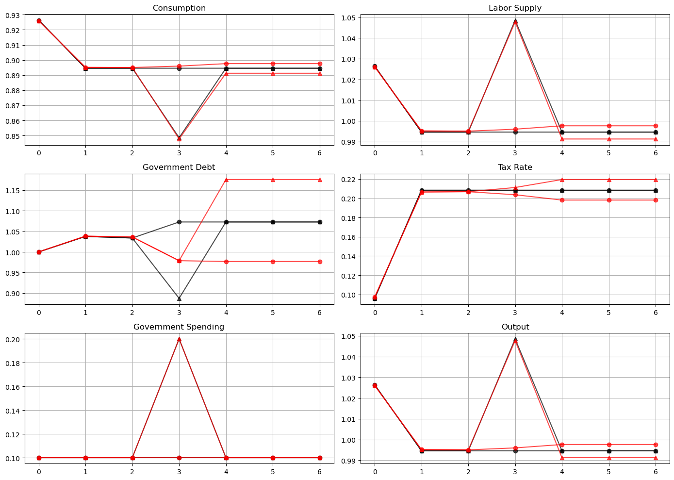
How a Ramsey planner responds to war depends on the structure of the asset market.
If it is able to trade state-contingent debt, then at time \(t=2\)
the government purchases an Arrow security that pays off when \(g_3 = g_h\)
the government sells an Arrow security that pays off when \(g_3 = g_l\)
the Ramsey planner designs these purchases and sales designed so that, regardless of whether or not there is a war at \(t=3\), the government begins period \(t=4\) with the same government debt
This pattern facilities smoothing tax rates across states.
The government without state-contingent debt cannot do this.
Instead, it must enter time \(t=3\) with the same level of debt falling due whether there is peace or war at \(t=3\).
The risk-free rate between time \(2\) and time \(3\) is unusually low because at time \(2\) consumption at time \(3\) is expected to be unusually low.
A low risk-free rate of return on government debt between time \(2\) and time \(3\) allows the government to enter period \(3\) with lower government debt than it entered period \(2\).
To finance a war at time \(3\) it raises taxes and issues more debt to carry into perpetual peace that begins in period \(4\).
To service the additional debt burden, it raises taxes in all future periods.
The absence of state-contingent debt leads to an important difference in the optimal tax policy.
When the Ramsey planner has access to state-contingent debt, the optimal tax policy is history independent
the tax rate is a function of the current level of government spending only, given the Lagrange multiplier on the implementability constraint
Without state-contingent debt, the optimal tax rate is history dependent.
A war at time \(t=3\) causes a permanent increase in the tax rate.
Peace at time \(t=3\) causes a permanent reduction in the tax rate.
55.4.1.1. Perpetual war alert#
History dependence occurs more dramatically in a case in which the government perpetually faces the prospect of war.
This case was studied in the final example of the lecture on optimal taxation with state-contingent debt.
There, each period the government faces a constant probability, \(0.5\), of war.
In addition, this example features the following preferences
In accordance, we will re-define our utility function.
log_util_data = [
    ('β', float64),
    ('ψ', float64)
]

@jitclass(log_util_data)
class LogUtility:

    def __init__(self,
                 β=0.9,
                 ψ=0.69):

        self.β, self.ψ = β, ψ

    # Utility function
    def U(self, c, l):
        return np.log(c) + self.ψ * np.log(l)

    # Derivatives of utility function
    def Uc(self, c, l):
        return 1 / c

    def Ucc(self, c, l):
        return -c**(-2)

    def Ul(self, c, l):
        return self.ψ / l

    def Ull(self, c, l):
        return -self.ψ / l**2

    def Ucl(self, c, l):
        return 0

    def Ulc(self, c, l):
        return 0
With these preferences, Ramsey tax rates will vary even in the Lucas-Stokey model with state-contingent debt.
The figure below plots optimal tax policies for both the economy with state-contingent debt (circles) and the economy with only a risk-free bond (triangles).
# WARNING: DO NOT EXPECT THE CODE TO WORK IF YOU CHANGE PARAMETERS
ψ = 0.69
Π = np.full((2, 2), 0.5)
β = 0.9
g = np.array([0.1, 0.2])

x_min = -3.4107
x_max = 3.709
x_num = 300

x_grid = [(x_min, x_max, x_num)]
log_pref = LogUtility(β=β, ψ=ψ)

S = len(Π)
bounds_v = np.vstack([np.zeros(2 * S), np.hstack([1 - g, np.ones(S)]) ]).T

V = np.zeros((len(Π), x_num))
V[:] = -(get_grid_nodes(x_grid[0]) + x_max) ** 2 / 14

σ_v_star = 1 - np.full((S, x_num, S * 2), 0.55)

W = np.empty(len(Π))
b_0 = 0.5
σ_w_star = 1 - np.full((S, 2), 0.55)

amss_model = AMSS(log_pref, β, Π, g, x_grid, bounds_v)
%%time

amss_model.solve(V, σ_v_star, b_0, W, σ_w_star, tol_vfi=3e-5, maxitr=3000,
                 print_itr=100)
===============
Solve time 1 problem
===============
Error at iteration 100 :  0.001156912305173563
Error at iteration 200 :  0.0005024950334071576
Error at iteration 300 :  0.0002995618583927495
Error at iteration 400 :  0.00020755613888212565
Error at iteration 500 :  0.00015558458529163488
Error at iteration 600 :  0.00012279319674135536
Error at iteration 700 :  0.00010068073823887858
Error at iteration 800 :  8.470541148142274e-05
Error at iteration 900 :  7.284396057016806e-05
Error at iteration 1000 :  6.370146950018807e-05
Error at iteration 1100 :  5.646858935470789e-05
Error at iteration 1200 :  5.048391475170888e-05
Error at iteration 1300 :  4.564400250117728e-05
Error at iteration 1400 :  4.146706198682182e-05
Error at iteration 1500 :  3.805415133761869e-05
Error at iteration 1600 :  3.521425495733865e-05
Error at iteration 1700 :  3.262771505951889e-05
Error at iteration 1800 :  3.0383804183742313e-05
Successfully completed VFI after 1819 iterations
===============
Solve time 0 problem
===============
Succesfully solved the time 0 problem.
CPU times: user 2min 6s, sys: 5.53 s, total: 2min 12s
Wall time: 1min 11s
ls_model = SequentialLS(log_pref, g=g, π=Π) # Solve sequential problem
# WARNING: DO NOT EXPECT THE CODE TO WORK IF YOU CHANGE PARAMETERS
s_hist = np.array([0, 0, 0, 0, 0, 0, 0, 0, 1, 1,
                   0, 0, 0, 1, 1, 1, 1, 1, 1, 0])

T = len(s_hist)

sim_amss = amss_model.simulate(s_hist, b_0)
sim_ls = ls_model.simulate(0.5, 0, T, s_hist)

titles = ['Consumption', 'Labor Supply', 'Government Debt',
          'Tax Rate', 'Government Spending', 'Output']

fig, axes = plt.subplots(3, 2, figsize=(14, 10))

for ax, title, ls, amss in zip(axes.flatten(), titles, sim_ls, sim_amss):
    ax.plot(ls, '-ok', amss, '-^b')
    ax.set(title=title)
    ax.grid()

axes[0, 0].legend(('Complete Markets', 'Incomplete Markets'))
plt.tight_layout()
plt.show()
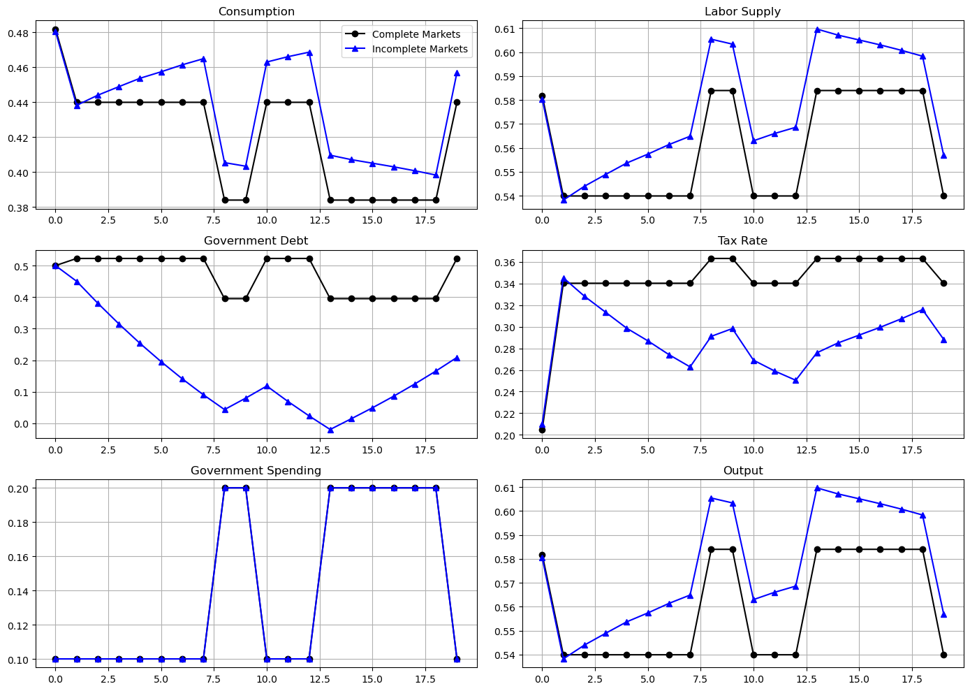
When the government experiences a prolonged period of peace, it is able to reduce government debt and set persistently lower tax rates.
However, the government finances a long war by borrowing and raising taxes.
This results in a drift away from policies with state-contingent debt that depends on the history of shocks.
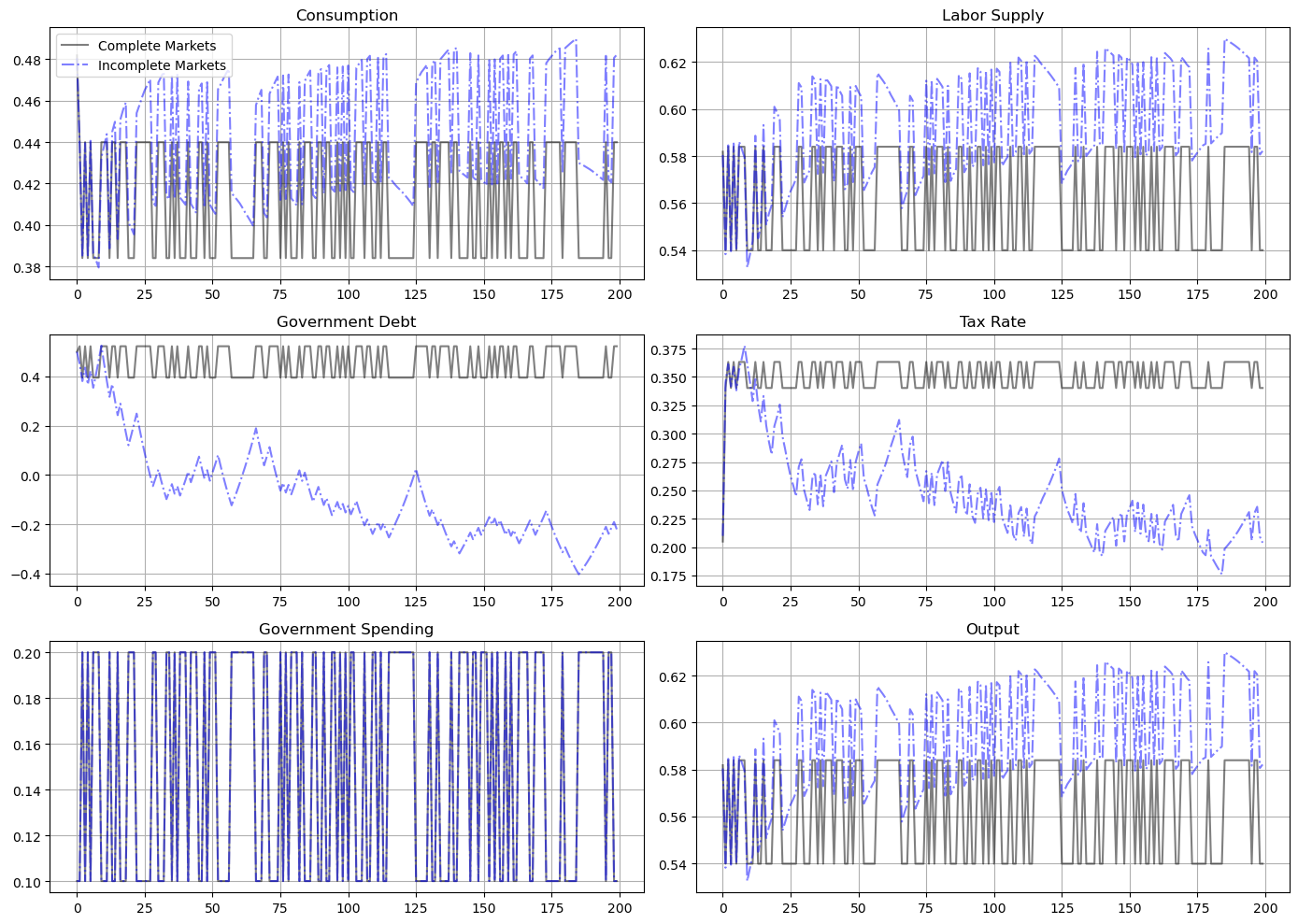
This is even more evident in the following figure that plots the evolution of the two policies over 200 periods.
This outcome reflects the presence of a force for precautionary saving that the incomplete markets structure imparts to the Ramsey plan.
In this subsequent lecture and this subsequent lecture, consequences of that force are explored.
T = 200
s_0 = 0
mc = MarkovChain(Π)

s_hist_long = mc.simulate(T, init=s_0, random_state=5)
sim_amss = amss_model.simulate(s_hist_long, b_0)
sim_ls = ls_model.simulate(0.5, 0, T, s_hist_long)

titles = ['Consumption', 'Labor Supply', 'Government Debt',
          'Tax Rate', 'Government Spending', 'Output']


fig, axes = plt.subplots(3, 2, figsize=(14, 10))

for ax, title, ls, amss in zip(axes.flatten(), titles, sim_ls, \
        sim_amss):
    ax.plot(ls, '-k', amss, '-.b', alpha=0.5)
    ax.set(title=title)
    ax.grid()

axes[0, 0].legend(('Complete Markets','Incomplete Markets'))
plt.tight_layout()
plt.show()