40. Stackelberg Plans#

In addition to what’s in Anaconda, this lecture will need the following libraries:

!pip install --upgrade quantecon

40.1. Overview#

This lecture formulates and computes a plan that a Stackelberg leader uses to manipulate forward-looking decisions of a Stackelberg follower that depend on continuation sequences of decisions made once and for all by the Stackelberg leader at time \(0\).

To facilitate computation and interpretation, we formulate things in a context that allows us to apply dynamic programming for linear-quadratic models.

Technically, our calculations are closely related to ones described this lecture.

From the beginning, we carry along a linear-quadratic model of duopoly in which firms face adjustment costs that make them want to forecast actions of other firms that influence future prices.

Let’s start with some standard imports:

import numpy as np
import numpy.linalg as la
import quantecon as qe
from quantecon import LQ
import matplotlib.pyplot as plt

40.2. Duopoly#

Time is discrete and is indexed by \(t = 0, 1, \ldots\).

Two firms produce a single good whose demand is governed by the linear inverse demand curve

\[ p_t = a_0 - a_1 (q_{1t}+ q_{2t} ) \]

where \(q_{it}\) is output of firm \(i\) at time \(t\) and \(a_0\) and \(a_1\) are both positive.

\(q_{10}, q_{20}\) are given numbers that serve as initial conditions at time \(0\).

By incurring a cost equal to

\[ \gamma v_{it}^2, \quad \gamma > 0 , \]

firm \(i\) can change its output according to

\[ q_{it+1} = q_{it} + v_{it} \]

Firm \(i\)’s profits at time \(t\) equal

\[ \pi_{it} = p_t q_{it} - \gamma v_{it}^2 \]

Firm \(i\) wants to maximize the present value of its profits

\[ \sum_{t=0}^\infty \beta^t \pi_{it} \]

where \(\beta \in (0,1)\) is a time discount factor.

40.2.1. Stackelberg Leader and Follower#

Each firm \(i=1,2\) chooses a sequence \(\vec q_i \equiv \{q_{it+1}\}_{t=0}^\infty\) once and for all at time \(0\).

We let firm 2 be a Stackelberg leader and firm 1 be a Stackelberg follower.

The leader firm 2 goes first and chooses \(\{q_{2t+1}\}_{t=0}^\infty\) once and for all at time \(0\).

Knowing that firm 2 has chosen \(\{q_{2t+1}\}_{t=0}^\infty\), the follower firm 1 goes second and chooses \(\{q_{1t+1}\}_{t=0}^\infty\) once and for all at time \(0\).

In choosing \(\vec q_2\), firm 2 takes into account that firm 1 will base its choice of \(\vec q_1\) on firm 2’s choice of \(\vec q_2\).

40.2.2. Statement of Leader’s and Follower’s Problems#

We can express firm 1’s problem as

\[ \max_{\vec q_1} \Pi_1(\vec q_1; \vec q_2) \]

where the appearance behind the semi-colon indicates that \(\vec q_2\) is given.

Firm 1’s problem induces the best response mapping

\[ \vec q_1 = B(\vec q_2) \]

(Here \(B\) maps a sequence into a sequence)

The Stackelberg leader’s problem is

\[ \max_{\vec q_2} \Pi_2 (B(\vec q_2), \vec q_2) \]

whose maximizer is a sequence \(\vec q_2\) that depends on the initial conditions \(q_{10}, q_{20}\) and the parameters of the model \(a_0, a_1, \gamma\).

This formulation captures key features of the model

Both firms make once-and-for-all choices at time \(0\).
This is true even though both firms are choosing sequences of quantities that are indexed by time.
The Stackelberg leader chooses first within time \(0\), knowing that the Stackelberg follower will choose second within time \(0\).

While our abstract formulation reveals the timing protocol and equilibrium concept well, it obscures details that must be addressed when we want to compute and interpret a Stackelberg plan and the follower’s best response to it.

To gain insights about these things, we study them in more detail.

40.2.3. Firms’ Problems#

Firm 1 acts as if firm 2’s sequence \(\{q_{2t+1}\}_{t=0}^\infty\) is given and beyond its control.

Firm 2 knows that firm 1 chooses second and takes this into account in choosing \(\{q_{2t+1}\}_{t=0}^\infty\).

In the spirit of working backward, we study firm 1’s problem first, taking \(\{q_{2t+1}\}_{t=0}^\infty\) as given.

We can formulate firm 1’s optimum problem in terms of the Lagrangian

\[ L=\sum_{t=0}^{\infty}\beta^{t}\{a_{0}q_{1t}-a_{1}q_{1t}^{2}-a_{1}q_{1t}q_{2t}-\gamma v_{1t}^{2}+\lambda_{t}[q_{1t}+v_{1t}-q_{1t+1}]\} \]

Firm 1 seeks a maximum with respect to \(\{q_{1t+1}, v_{1t} \}_{t=0}^\infty\) and a minimum with respect to \(\{ \lambda_t\}_{t=0}^\infty\).

We approach this problem using methods described in [Ljungqvist and Sargent, 2018], chapter 2, appendix A and [Sargent, 1987], chapter IX.

First-order conditions for this problem are

\[ \begin{aligned} \frac{\partial L}{\partial q_{1t}} & = a_0 - 2 a_1 q_{1t} - a_1 q_{2t} + \lambda_t - \beta^{-1} \lambda_{t-1} = 0 , \quad t \geq 1 \cr \frac{\partial L}{\partial v_{1t}} & = -2 \gamma v_{1t} + \lambda_t = 0 , \quad t \geq 0 \cr \end{aligned} \]

These first-order conditions and the constraint \(q_{1t+1} = q_{1t} + v_{1t}\) can be rearranged to take the form

\[ \begin{aligned} v_{1t} & = \beta v_{1t+1} + \frac{\beta a_0}{2 \gamma} - \frac{\beta a_1}{\gamma} q_{1t+1} - \frac{\beta a_1}{2 \gamma} q_{2t+1} \cr q_{t+1} & = q_{1t} + v_{1t} \end{aligned} \]

We can substitute the second equation into the first equation to obtain

\[ (q_{1t+1} - q_{1t} ) = \beta (q_{1t+2} - q_{1t+1}) + c_0 - c_1 q_{1t+1} - c_2 q_{2t+1} \]

where \(c_0 = \frac{\beta a_0}{2 \gamma}, c_1 = \frac{\beta a_1}{\gamma}, c_2 = \frac{\beta a_1}{2 \gamma}\).

This equation can in turn be rearranged to become

(40.1)#\[- q_{1t} + (1+\beta + c_1) q_{1t+1} - \beta q_{1t+2} = c_0 - c_2 q_{2t+1}\]

Equation (40.1) is a second-order difference equation in the sequence \(\vec q_1\) whose solution we want.

It satisfies two boundary conditions:

an initial condition that \(q_{1,0}\), which is given
a terminal condition requiring that \(\lim_{T \rightarrow + \infty} \beta^T q_{1t}^2 < + \infty\)

Using the lag operators described in [Sargent, 1987], chapter IX, difference equation (40.1) can be written as

\[ \beta(1 - \frac{1+\beta + c_1}{\beta} L + \beta^{-1} L^2 ) q_{1t+2} = - c_0 + c_2 q_{2t+1} \]

The polynomial in the lag operator on the left side can be factored as

(40.2)#\[(1 - \frac{1+\beta + c_1}{\beta} L + \beta^{-1} L^2 ) = ( 1 - \delta_1 L ) (1 - \delta_2 L)\]

where \(0 < \delta_1 < 1 < \frac{1}{\sqrt{\beta}} < \delta_2\).

Because \(\delta_2 > \frac{1}{\sqrt{\beta}}\) the operator \((1 - \delta_2 L)\) contributes an unstable component if solved backwards but a stable component if solved forwards.

Mechanically, write

\[ (1- \delta_2 L) = -\delta_{2} L (1 - \delta_2^{-1} L^{-1} ) \]

and compute the following inverse operator

\[ \left[-\delta_{2} L (1 - \delta_2^{-1} L^{-1} )\right]^{-1} = - \delta_2 (1 - {\delta_2}^{-1} )^{-1} L^{-1} \]

Operating on both sides of equation (40.2) with \(\beta^{-1}\) times this inverse operator gives the follower’s decision rule for setting \(q_{1t+1}\) in the feedback-feedforward form

(40.3)#\[q_{1t+1} = \delta_1 q_{1t} - c_0 \delta_2^{-1} \beta^{-1} \frac{1}{1 -\delta_2^{-1}} + c_2 \delta_2^{-1} \beta^{-1} \sum_{j=0}^\infty \delta_2^j q_{2t+j+1} , \quad t \geq 0\]

The problem of the Stackelberg leader firm 2 is to choose the sequence \(\{q_{2t+1}\}_{t=0}^\infty\) to maximize its discounted profits

\[ \sum_{t=0}^\infty \beta^t \{ (a_0 - a_1 (q_{1t} + q_{2t}) ) q_{2t} - \gamma (q_{2t+1} - q_{2t})^2 \} \]

subject to the sequence of constraints (40.3) for \(t \geq 0\).

We can put a sequence \(\{\theta_t\}_{t=0}^\infty\) of Lagrange multipliers on the sequence of equations (40.3) and formulate the following Lagrangian for the Stackelberg leader firm 2’s problem

(40.4)#\[\begin{aligned} \tilde L & = \sum_{t=0}^\infty \beta^t\{ (a_0 - a_1 (q_{1t} + q_{2t}) ) q_{2t} - \gamma (q_{2t+1} - q_{2t})^2 \} \cr & + \sum_{t=0}^\infty \beta^t \theta_t \{ \delta_1 q_{1t} - c_0 \delta_2^{-1} \beta^{-1} \frac{1}{1 -\delta_2^{-1}} + c_2 \delta_2^{-1} \beta^{-1} \sum_{j=0}^\infty \delta_2^{-j} q_{2t+j+1} - q_{1t+1} \} \end{aligned}\]

subject to initial conditions for \(q_{1t}, q_{2t}\) at \(t=0\).

Remarks: We have formulated the Stackelberg problem in a space of sequences.

The max-min problem associated with firm 2’s Lagrangian (40.4) is unpleasant because the time \(t\) component of firm \(2\)’s payoff function depends on the entire future of its choices of \(\{q_{2t+j}\}_{j=0}^\infty\).

This renders a direct attack on the problem in the space of sequences cumbersome.

Therefore, below we will formulate the Stackelberg leader’s problem recursively.

We’ll proceed by putting our duopoly model into a broader class of models with the same general structure.

40.3. Stackelberg Problem#

We formulate a class of linear-quadratic Stackelberg leader-follower problems of which our duopoly model is an instance.

We use the optimal linear regulator (a.k.a. the linear-quadratic dynamic programming problem described in LQ Dynamic Programming problems) to represent a Stackelberg leader’s problem recursively.

Let \(z_t\) be an \(n_z \times 1\) vector of natural state variables.

Let \(x_t\) be an \(n_x \times 1\) vector of endogenous forward-looking variables that are physically free to jump at \(t\).

In our duopoly example \(x_t = v_{1t}\), the time \(t\) decision of the Stackelberg follower.

Let \(u_t\) be a vector of decisions chosen by the Stackelberg leader at \(t\).

The \(z_t\) vector is inherited from the past.

But \(x_t\) is a decision made by the Stackelberg follower at time \(t\) that is the follower’s best response to the choice of an entire sequence of decisions made by the Stackelberg leader at time \(t=0\).

Let

\[\begin{split} y_t = \begin{bmatrix} z_t \\ x_t \end{bmatrix} \end{split}\]

Represent the Stackelberg leader’s one-period loss function as

\[ r(y, u) = y' R y + u' Q u \]

Subject to an initial condition for \(z_0\), but not for \(x_0\), the Stackelberg leader wants to maximize

(40.5)#\[-\sum_{t=0}^\infty \beta^t r(y_t, u_t)\]

The Stackelberg leader faces the model

(40.6)#\[\begin{split}\begin{bmatrix} I & 0 \\ G_{21} & G_{22} \end{bmatrix} \begin{bmatrix} z_{t+1} \\ x_{t+1} \end{bmatrix} = \begin{bmatrix} \hat A_{11} & \hat A_{12} \\ \hat A_{21} & \hat A_{22} \end{bmatrix} \begin{bmatrix} z_t \\ x_t \end{bmatrix} + \hat B u_t\end{split}\]

We assume that the matrix \(\begin{bmatrix} I & 0 \\ G_{21} & G_{22} \end{bmatrix}\) on the left side of equation (40.6) is invertible, so that we can multiply both sides by its inverse to obtain

(40.7)#\[\begin{split}\begin{bmatrix} z_{t+1} \\ x_{t+1} \end{bmatrix} = \begin{bmatrix} A_{11} & A_{12} \\ A_{21} & A_{22} \end{bmatrix} \begin{bmatrix} z_t \\ x_t \end{bmatrix} + B u_t\end{split}\]

(40.8)#\[y_{t+1} = A y_t + B u_t\]

40.3.1. Interpretation of Second Block of Equations#

The Stackelberg follower’s best response mapping is summarized by the second block of equations of (40.7).

In particular, these equations are the first-order conditions of the Stackelberg follower’s optimization problem (i.e., its Euler equations).

These Euler equations summarize the forward-looking aspect of the follower’s behavior and express how its time \(t\) decision depends on the leader’s actions at times \(s \geq t\).

When combined with a stability condition to be imposed below, the Euler equations summarize the follower’s best response to the sequence of actions by the leader.

The Stackelberg leader maximizes (40.5) by choosing sequences \(\{u_t, x_t, z_{t+1}\}_{t=0}^{\infty}\) subject to (40.8) and an initial condition for \(z_0\).

Note that we have an initial condition for \(z_0\) but not for \(x_0\).

\(x_0\) is among the variables to be chosen at time \(0\) by the Stackelberg leader.

The Stackelberg leader uses its understanding of the responses restricted by (40.8) to manipulate the follower’s decisions.

40.3.2. More Mechanical Details#

For any vector \(a_t\), define \(\vec a_t = [a_t, a_{t+1} \ldots ]\).

Define a feasible set of \((\vec y_1, \vec u_0)\) sequences

\[ \Omega(y_0) = \left\{ (\vec y_1, \vec u_0) : y_{t+1} = A y_t + B u_t, \forall t \geq 0 \right\} \]

Please remember that the follower’s system of Euler equations is embedded in the system of dynamic equations \(y_{t+1} = A y_t + B u_t\).

Note that the definition of \(\Omega(y_0)\) treats \(y_0\) as given.

Although it is taken as given in \(\Omega(y_0)\), eventually, the \(x_0\) component of \(y_0\) is to be chosen by the Stackelberg leader.

40.3.3. Two Subproblems#

Once again we use backward induction.

We express the Stackelberg problem in terms of two subproblems.

Subproblem 1 is solved by a continuation Stackelberg leader at each date \(t \geq 0\).

Subproblem 2 is solved by the Stackelberg leader at \(t=0\).

The two subproblems are designed

to respect the timing protocol in which the follower chooses \(\vec q_1\) after seeing \(\vec q_2\) chosen by the leader
to make the leader choose \(\vec q_2\) while respecting that \(\vec q_1\) will be the follower’s best response to \(\vec q_2\)
to represent the leader’s problem recursively by artfully choosing the leader’s state variables and the control variables available to the leader

Subproblem 1

\[ v(y_0) = \max_{(\vec y_1, \vec u_0) \in \Omega(y_0)} - \sum_{t=0}^\infty \beta^t r(y_t, u_t) \]

Subproblem 2

\[ w(z_0) = \max_{x_0} v(y_0) \]

Subproblem 1 takes the vector of forward-looking variables \(x_0\) as given.

Subproblem 2 optimizes over \(x_0\).

The value function \(w(z_0)\) tells the value of the Stackelberg plan as a function of the vector of natural state variables \(z_0\) at time \(0\).

40.4. Two Bellman Equations#

We now describe Bellman equations for \(v(y)\) and \(w(z_0)\).

Subproblem 1

The value function \(v(y)\) in subproblem 1 satisfies the Bellman equation

(40.9)#\[v(y) = \max_{u, y^*} \left\{ - r(y,u) + \beta v(y^*) \right\}\]

where the maximization is subject to

\[ y^* = A y + B u \]

and \(y^*\) denotes next period’s value.

Substituting \(v(y) = - y'P y\) into Bellman equation (40.9) gives

\[ -y' P y = {\rm max}_{ u, y^*} \left\{ - y' R y - u'Q u - \beta y^{* \prime} P y^* \right\} \]

which as in lecture linear regulator gives rise to the algebraic matrix Riccati equation

\[ P = R + \beta A' P A - \beta^2 A' P B ( Q + \beta B' P B)^{-1} B' P A \]

and the optimal decision rule coefficient vector

\[ F = \beta( Q + \beta B' P B)^{-1} B' P A \]

where the optimal decision rule is

\[ u_t = - F y_t \]

Subproblem 2

We find an optimal \(x_0\) by equating to zero the gradient of \(v(y_0)\) with respect to \(x_0\):

\[ -2 P_{21} z_0 - 2 P_{22} x_0 =0, \]

which implies that

(40.10)#\[ x_0 = - P_{22}^{-1} P_{21} z_0 \]

40.5. Stackelberg Plan for Duopoly#

Now let’s map our duopoly model into the above setup.

We formulate a state vector

\[ y_t = \begin{bmatrix} z_t \cr x_t \end{bmatrix} \]

where for our duopoly model

\[ z_t = \begin{bmatrix} 1 \cr q_{2t} \cr q_{1t} \end{bmatrix} , \quad x_t = v_{1t}, \]

where \(x_t = v_{1t}\) is the time \(t\) decision of the follower firm 1, \(u_t\) is the time \(t\) decision of the leader firm 2 and

\[ v_{1t} = q_{1t+1} - q_{1t}, \quad u_t = q_{2t+1} - q_{2t} . \]

For our duopoly model, initial conditions for the natural state variables in \(z_t\) are

\[ z_0 = \begin{bmatrix} 1 \cr q_{20} \cr q_{10} \end{bmatrix} \]

while \(x_0 = v_{10} = q_{11} - q_{10}\) is a choice variable for the Stackelberg leader firm 2, one that will ultimately be chosen according an optimal rule prescribed by (40.10) for subproblem 2 above.

That the Stackelberg leader firm 2 chooses \(x_0 = v_{10}\) is subtle.

Of course, \(x_0 = v_{10}\) emerges from the feedback-feedforward solution (40.3) of firm 1’s system of Euler equations, so that it is actually firm 1 that sets \(x_0\).

But firm 2 manipulates firm 1’s choice through firm 2’s choice of the sequence \(\vec q_{2,1} = \{q_{2t+1}\}_{t=0}^\infty\).

40.5.1. Calculations to Prepare Duopoly Model#

Now we’ll proceed to cast our duopoly model within the framework of the more general linear-quadratic structure described above.

That will allow us to compute a Stackelberg plan simply by enlisting a Riccati equation to solve a linear-quadratic dynamic program.

As emphasized above, firm 1 acts as if firm 2’s decisions \(\{q_{2t+1}, v_{2t}\}_{t=0}^\infty\) are given and beyond its control.

40.5.2. Firm 1’s Problem#

We again formulate firm 1’s optimum problem in terms of the Lagrangian

\[ L=\sum_{t=0}^{\infty}\beta^{t}\{a_{0}q_{1t}-a_{1}q_{1t}^{2}-a_{1}q_{1t}q_{2t}-\gamma v_{1t}^{2}+\lambda_{t}[q_{1t}+v_{1t}-q_{1t+1}]\} \]

Firm 1 seeks a maximum with respect to \(\{q_{1t+1}, v_{1t} \}_{t=0}^\infty\) and a minimum with respect to \(\{ \lambda_t\}_{t=0}^\infty\).

First-order conditions for this problem are

These first-order order conditions and the constraint \(q_{1t+1} = q_{1t} + v_{1t}\) can be rearranged to take the form

\[ \begin{aligned} v_{1t} & = \beta v_{1t+1} + \frac{\beta a_0}{2 \gamma} - \frac{\beta a_1}{\gamma} q_{1t+1} - \frac{\beta a_1}{2 \gamma} q_{2t+1} \cr q_{t+1} & = q_{1t} + v_{1t} \end{aligned} \]

We use these two equations as components of the following linear system that confronts a Stackelberg continuation leader at time \(t\)

\[ \begin{bmatrix} 1 & 0 & 0 & 0 \cr 0 & 1 & 0 & 0 \cr 0 & 0 & 1 & 0 \cr \frac{\beta a_0}{2 \gamma} & - \frac{\beta a_1}{2 \gamma} & -\frac{\beta a_1}{\gamma} & \beta \end{bmatrix} \begin{bmatrix} 1 \cr q_{2t+1} \cr q_{1t+1} \cr v_{1t+1} \end{bmatrix} = \begin{bmatrix} 1 & 0 & 0 & 0 \cr 0 & 1 & 0 & 0 \cr 0 & 0 & 1 & 1 \cr 0 & 0 & 0 & 1 \end{bmatrix} \begin{bmatrix} 1 \cr q_{2t} \cr q_{1t} \cr v_{1t} \end{bmatrix} + \begin{bmatrix} 0 \cr 1 \cr 0 \cr 0 \end{bmatrix} v_{2t} \]

Time \(t\) revenues of firm 2 are \(\pi_{2t} = a_0 q_{2t} - a_1 q_{2t}^2 - a_1 q_{1t} q_{2t}\) which evidently equal

\[ z_t' R_1 z_t \equiv \begin{bmatrix} 1 \cr q_{2t} \cr q_{1t} \end{bmatrix}' \begin{bmatrix} 0 & \frac{a_0}{2}& 0 \cr \frac{a_0}{2} & -a_1 & -\frac{a_1}{2}\cr 0 & -\frac{a_1}{2} & 0 \end{bmatrix} \begin{bmatrix} 1 \cr q_{2t} \cr q_{1t} \end{bmatrix} \]

If we set \(Q = \gamma\), then firm 2’s period \(t\) profits can then be written

\[ y_t' R y_t - Q v_{2t}^2 \]

where

\[ y_t = \begin{bmatrix} z_t \cr x_t \end{bmatrix} \]

with \(x_t = v_{1t}\) and

\[ R = \begin{bmatrix} R_1 & 0 \cr 0 & 0 \end{bmatrix} \]

We’ll report results of implementing this code soon.

But first, we want to represent the Stackelberg leader’s optimal choices recursively.

It is important to do this for several reasons:

properly to interpret a representation of the Stackelberg leader’s choice as a sequence of history-dependent functions
to formulate a recursive version of the follower’s choice problem

First, let’s get a recursive representation of the Stackelberg leader’s choice of \(\vec q_2\) for our duopoly model.

40.6. Recursive Representation of Stackelberg Plan#

In order to attain an appropriate representation of the Stackelberg leader’s history-dependent plan, we will employ what amounts to a version of the Big K, little k device often used in macroeconomics by distinguishing \(z_t\), which depends partly on decisions \(x_t\) of the followers, from another vector \(\check z_t\), which does not.

We will use \(\check z_t\) and its history \(\check z^t = [\check z_t, \check z_{t-1}, \ldots, \check z_0]\) to describe the sequence of the Stackelberg leader’s decisions that the Stackelberg follower takes as given.

Thus, we let \(\check y_t' = \begin{bmatrix}\check z_t' & \check x_t'\end{bmatrix}\) with initial condition \(\check z_0 = z_0\) given.

That we distinguish \(\check z_t\) from \(z_t\) is part and parcel of the Big K, little k device in this instance.

We have demonstrated that a Stackelberg plan for \(\{u_t\}_{t=0}^\infty\) has a recursive representation

\[ \begin{aligned} \check x_0 & = - P_{22}^{-1} P_{21} z_0 \cr u_t & = - F \check y_t, \quad t \geq 0 \cr \check y_{t+1} & = (A - BF) \check y_t, \quad t \geq 0 \end{aligned} \]

From this representation, we can deduce the sequence of functions \(\sigma = \{\sigma_t(\check z^t)\}_{t=0}^\infty\) that comprise a Stackelberg plan.

For convenience, let \(\check A \equiv A - BF\) and partition \(\check A\) conformably to the partition \(y_t = \begin{bmatrix}\check z_t \cr \check x_t \end{bmatrix}\) as

\[ \begin{bmatrix}\check A_{11} & \check A_{12} \cr \check A_{21} & \check A_{22} \end{bmatrix} \]

Let \(H^0_0 \equiv - P_{22}^{-1} P_{21}\) so that \(\check x_0 = H^0_0 \check z_0\).

Then iterations on \(\check y_{t+1} = \check A \check y_t\) starting from initial condition \(\check y_0 = \begin{bmatrix}\check z_0 \cr H^0_0 \check z_0\end{bmatrix}\) imply that for \(t \geq 1\)

\[ \check x_t = \sum_{j=1}^t H_j^t \check z_{t-j} \]

where

\[ \begin{aligned} H^t_1 & = \check A_{21} \cr H^t_2 & = \check A_{22} \check A_{21} \cr \ \ \vdots \ \ & \ \ \quad \vdots \cr H^t_{t-1} & = \check A_{22}^{t-2} \check A_{21} \cr H^t_t & = \check A_{22}^{t-1}(\check A_{21} + \check A_{22} H^0_0 ) \end{aligned} \]

An optimal decision rule for the Stackelberg leader’s choice of \(u_t\) is

\[ u_t = - F \check y_t \equiv - \begin{bmatrix} F_z & F_x \cr \end{bmatrix} \begin{bmatrix}\check z_t \cr x_t \cr \end{bmatrix} \]

(40.11)#\[u_t = - F_z \check z_t - F_x \sum_{j=1}^t H^t_j z_{t-j} = \sigma_t(\check z^t)\]

Representation (40.11) confirms that whenever \(F_x \neq 0\), the typical situation, the time \(t\) component \(\sigma_t\) of a Stackelberg plan is history-dependent, meaning that the Stackelberg leader’s choice \(u_t\) depends not just on \(\check z_t\) but on components of \(\check z^{t-1}\).

40.6.1. Comments and Interpretations#

Because we set \(\check z_0 = z_0\), it will turn out that \(z_t = \check z_t\) for all \(t \geq 0\).

Then why did we distinguish \(\check z_t\) from \(z_t\)?

The answer is that if we want to present to the Stackelberg follower a history-dependent representation of the Stackelberg leader’s sequence \(\vec q_2\), we must use representation (40.11) cast in terms of the history \(\check z^t\) and not a corresponding representation cast in terms of \(z^t\).

40.7. Dynamic Programming and Time Consistency of Follower’s Problem#

Given the sequence \(\vec q_2\) chosen by the Stackelberg leader in our duopoly model, it turns out that the Stackelberg follower’s problem is recursive in the natural state variables that confront a follower at any time \(t \geq 0\).

This means that the follower’s plan is time consistent.

To verify these claims, we’ll formulate a recursive version of a follower’s problem that builds on our recursive representation of the Stackelberg leader’s plan and our use of the Big K, little k idea.

40.7.1. Recursive Formulation of a Follower’s Problem#

We now use what amounts to another “Big \(K\), little \(k\)” trick (see rational expectations equilibrium) to formulate a recursive version of a follower’s problem cast in terms of an ordinary Bellman equation.

Firm 1, the follower, faces \(\{q_{2t}\}_{t=0}^\infty\) as a given quantity sequence chosen by the leader and believes that its output price at \(t\) satisfies

\[ p_t = a_0 - a_1 ( q_{1t} + q_{2t}) , \quad t \geq 0 \]

Our challenge is to represent \(\{q_{2t}\}_{t=0}^\infty\) as a given sequence.

To do so, recall that under the Stackelberg plan, firm 2 sets output according to the \(q_{2t}\) component of

\[ y_{t+1} = \begin{bmatrix} 1 \cr q_{2t} \cr q_{1t} \cr x_t \end{bmatrix} \]

which is governed by

\[ y_{t+1} = (A - BF) y_t \]

To obtain a recursive representation of a \(\{q_{2t}\}\) sequence that is exogenous to firm 1, we define a state \(\tilde y_t\)

\[ \tilde y_t = \begin{bmatrix} 1 \cr q_{2t} \cr \tilde q_{1t} \cr \tilde x_t \end{bmatrix} \]

that evolves according to

\[ \tilde y_{t+1} = (A - BF) \tilde y_t \]

subject to the initial condition \(\tilde q_{10} = q_{10}\) and \(\tilde x_0 = x_0\) where \(x_0 = - P_{22}^{-1} P_{21}\) as stated above.

Firm 1’s state vector is

\[ X_t = \begin{bmatrix} \tilde y_t \cr q_{1t} \end{bmatrix} \]

It follows that the follower firm 1 faces law of motion

(40.12)#\[\begin{split}\begin{bmatrix} \tilde y_{t+1} \\ q_{1t+1} \end{bmatrix} = \begin{bmatrix} A - BF & 0 \\ 0 & 1 \end{bmatrix} \begin{bmatrix} \tilde y_{t} \\ q_{1t} \end{bmatrix} + \begin{bmatrix} 0 \cr 1 \end{bmatrix} x_t\end{split}\]

This specification assures that from the point of the view of firm 1, \(q_{2t}\) is an exogenous process.

Here

\(\tilde q_{1t}, \tilde x_t\) play the role of Big K
\(q_{1t}, x_t\) play the role of little k

The time \(t\) component of firm 1’s objective is

\[ \tilde X_t' \tilde R x_t - x_t^2 \tilde Q = \begin{bmatrix} 1 \cr q_{2t} \cr \tilde q_{1t} \cr \tilde x_t \cr q_{1t} \end{bmatrix}' \begin{bmatrix} 0 & 0 & 0 & 0 & \frac{a_0}{2} \cr 0 & 0 & 0 & 0 & - \frac{a_1}{2} \cr 0 & 0 & 0 & 0 & 0 \cr 0 & 0 & 0 & 0 & 0 \cr \frac{a_0}{2} & -\frac{a_1}{2} & 0 & 0 & - a_1 \end{bmatrix} \begin{bmatrix} 1 \cr q_{2t} \cr \tilde q_{1t} \cr \tilde x_t \cr q_{1t} \end{bmatrix} - \gamma x_t^2 \]

Firm 1’s optimal decision rule is

\[ x_t = - \tilde F X_t \]

and its state evolves according to

\[ \tilde X_{t+1} = (\tilde A - \tilde B \tilde F) X_t \]

under its optimal decision rule.

Later we shall compute \(\tilde F\) and verify that when we set

\[ X_0 = \begin{bmatrix} 1 \cr q_{20} \cr q_{10} \cr x_0 \cr q_{10} \end{bmatrix} \]

we recover

\[ x_0 = - \tilde F \tilde X_0 , \]

which will verify that we have properly set up a recursive representation of the follower’s problem facing the Stackelberg leader’s \(\vec q_2\).

40.7.2. Time Consistency of Follower’s Plan#

The follower can solve its problem using dynamic programming because its problem is recursive in what for it are the natural state variables, namely

\[ \begin{bmatrix} 1 \cr q_{2t} \cr \tilde q_{1t} \cr \tilde x_t \end{bmatrix} \]

It follows that the follower’s plan is time consistent.

40.8. Computing Stackelberg Plan#

Here is our code to compute a Stackelberg plan via the linear-quadratic dynamic program describe above.

Let’s use it to compute the Stackelberg plan.

# Parameters
a0 = 10
a1 = 2
β = 0.96
γ = 120
n = 300
tol0 = 1e-8
tol1 = 1e-16
tol2 = 1e-2

βs = np.ones(n)
βs[1:] = β
βs = βs.cumprod()

# In LQ form
Alhs = np.eye(4)

# Euler equation coefficients
Alhs[3, :] = β * a0 / (2 * γ), -β * a1 / (2 * γ), -β * a1 / γ, β

Arhs = np.eye(4)
Arhs[2, 3] = 1

Alhsinv = la.inv(Alhs)

A = Alhsinv @ Arhs

B = Alhsinv @ np.array([[0, 1, 0, 0]]).T

R = np.array([[0,      -a0 / 2,      0, 0],
              [-a0 / 2,     a1, a1 / 2, 0],
              [0,       a1 / 2,      0, 0],
              [0,            0,      0, 0]])

Q = np.array([[γ]])

# Solve using QE's LQ class
# LQ solves minimization problems which is why the sign of R and Q was changed
lq = LQ(Q, R, A, B, beta=β)
P, F, d = lq.stationary_values(method='doubling')

P22 = P[3:, 3:]
P21 = P[3:, :3]
P22inv = la.inv(P22)
H_0_0 = -P22inv @ P21

# Simulate forward

π_leader = np.zeros(n)

z0 = np.array([[1, 1, 1]]).T
x0 = H_0_0 @ z0
y0 = np.vstack((z0, x0))

yt, ut = lq.compute_sequence(y0, ts_length=n)[:2]

π_matrix = (R + F. T @ Q @ F)

for t in range(n):
    π_leader[t] = -(yt[:, t].T @ π_matrix @ yt[:, t])

# Display policies
print("Computed policy for Continuation Stackelberg leader\n")
print(f"F = {F}")

Computed policy for Continuation Stackelberg leader

F = [[-1.58004454  0.29461313  0.67480938  6.53970594]]

40.9. Time Series for Price and Quantities#

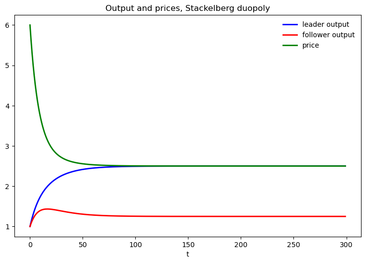
Now let’s use the code to compute and display outcomes as a Stackelberg plan unfolds.

The following code plots quantities chosen by the Stackelberg leader and follower, together with the equilibrium output price.

q_leader = yt[1, :-1]
q_follower = yt[2, :-1]
q = q_leader + q_follower       # Total output, Stackelberg
p = a0 - a1 * q                 # Price, Stackelberg

fig, ax = plt.subplots(figsize=(9, 5.8))
ax.plot(range(n), q_leader, 'b-', lw=2, label='leader output')
ax.plot(range(n), q_follower, 'r-', lw=2, label='follower output')
ax.plot(range(n), p, 'g-', lw=2, label='price')
ax.set_title('Output and prices, Stackelberg duopoly')
ax.legend(frameon=False)
ax.set_xlabel('t')
plt.show()

_images/a750e456054f7c826be81f95ae4cfb3f6a1e789ee47e193f39e4a35a8a744c3a.png

40.9.1. Value of Stackelberg Leader#

We’ll compute the value \(w(x_0)\) attained by the Stackelberg leader, where \(x_0\) is given by the maximizer (40.10) of subproblem 2.

We’ll compute it two ways and get the same answer.

In addition to being a useful check on the accuracy of our coding, computing things in these two ways helps us think about the structure of the problem.

v_leader_forward = np.sum(βs * π_leader)
v_leader_direct = -yt[:, 0].T @ P @ yt[:, 0]

# Display values
print("Computed values for the Stackelberg leader at t=0:\n")
print(f"v_leader_forward(forward sim) = {v_leader_forward:.4f}")
print(f"v_leader_direct (direct) = {v_leader_direct:.4f}")

Computed values for the Stackelberg leader at t=0:

v_leader_forward(forward sim) = 150.0316
v_leader_direct (direct) = 150.0324

# Manually checks whether P is approximately a fixed point
P_next = (R + F.T @ Q @ F + β * (A - B @ F).T @ P @ (A - B @ F))
(P - P_next < tol0).all()

True

# Manually checks whether two different ways of computing the
# value function give approximately the same answer
v_expanded = -((y0.T @ R @ y0 + ut[:, 0].T @ Q @ ut[:, 0] +
               β * (y0.T @ (A - B @ F).T @ P @ (A - B @ F) @ y0)))
(v_leader_direct - v_expanded < tol0)[0, 0]

True

40.10. Time Inconsistency of Stackelberg Plan#

In the code below we compare two values

the continuation value \(v(y_t) = - y_t' P y_t\) earned by a continuation Stackelberg leader who inherits state \(y_t\) at \(t\)
the value \(w(\hat x_t)\) of a reborn Stackelberg leader who, at date \(t\) along the Stackelberg plan, inherits state \(z_t\) at \(t\) but who discards \(x_t\) from the time \(t\) continuation of the original Stackelberg plan and resets it to \( \hat x_t = - P_{22}^{-1} P_{21} z_t\)

The difference between these two values is a tell-tale sign of the time inconsistency of the Stackelberg plan

# Compute value function over time with a reset at time t
vt_leader = np.zeros(n)
vt_reset_leader = np.empty_like(vt_leader)

yt_reset = yt.copy()
yt_reset[-1, :] = (H_0_0 @ yt[:3, :])

for t in range(n):
    vt_leader[t] = -yt[:, t].T @ P @ yt[:, t]
    vt_reset_leader[t] = -yt_reset[:, t].T @ P @ yt_reset[:, t]

fig, axes = plt.subplots(3, 1, figsize=(10, 7))

axes[0].plot(range(n+1), (- F @ yt).flatten(), 'bo',
    label='Stackelberg leader', ms=2)
axes[0].plot(range(n+1), (- F @ yt_reset).flatten(), 'ro',
    label='reborn  at t Stackelberg leader', ms=2)
axes[0].set(title=r' $u_{t} = q_{2t+1} - q_t$', xlabel='t')
axes[0].legend()

axes[1].plot(range(n+1), yt[3, :], 'bo', ms=2)
axes[1].plot(range(n+1), yt_reset[3, :], 'ro', ms=2)
axes[1].set(title=r' $x_{t} = q_{1t+1} - q_{1t}$', xlabel='t')

axes[2].plot(range(n), vt_leader, 'bo', ms=2)
axes[2].plot(range(n), vt_reset_leader, 'ro', ms=2)
axes[2].set(title=r'$v(y_{t})$ and $w(\hat x_t)$', xlabel='t')

plt.tight_layout()
plt.show()

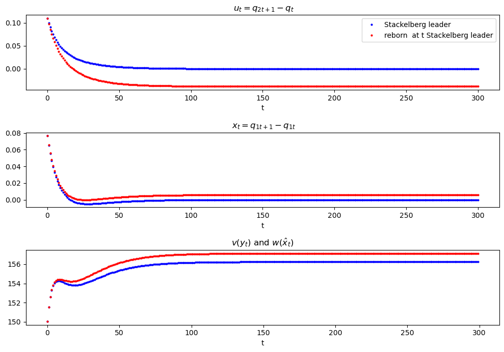
_images/544813ce98ba0acfb0101a7f5f0c702396d3ea6d61cdb66d667368a3f13f5d5e.png

The figure above shows

in the third panel that for \(t \geq 1\) the reborn at \(t\) Stackelberg leader’s’s value \(w(\hat x_0)\) exceeds the continuation value \(v(y_t)\) of the time \(0\) Stackelberg leader
in the first panel that for \(t \geq 1\) the reborn at \(t\) Stackelberg leader wants to reduce his output below that prescribed by the time \(0\) Stackelberg leader
in the second panel that for \(t \geq 1\) the reborn at \(t\) Stackelberg leader wants to increase the output of the follower firm 2 below that prescribed by the time \(0\) Stackelberg leader

Taken together, these outcomes express the time inconsistency of the original time \(0\) Stackelberg leaders’s plan.

40.11. Recursive Formulation of Follower’s Problem#

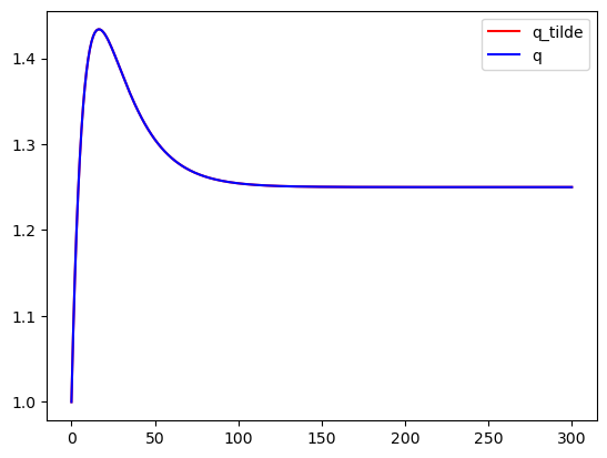
We now formulate and compute the recursive version of the follower’s problem.

We check that the recursive Big \(K\) , little \(k\) formulation of the follower’s problem produces the same output path \(\vec q_1\) that we computed when we solved the Stackelberg problem

A_tilde = np.eye(5)
A_tilde[:4, :4] = A - B @ F

R_tilde = np.array([[0,            0, 0,    0, -a0 / 2],
                    [0,            0, 0,    0,  a1 / 2],
                    [0,            0, 0,    0,       0],
                    [0,            0, 0,    0,       0],
                    [-a0 / 2, a1 / 2, 0,    0,      a1]])

Q_tilde = Q
B_tilde = np.array([[0, 0, 0, 0, 1]]).T

lq_tilde = LQ(Q_tilde, R_tilde, A_tilde, B_tilde, beta=β)
P_tilde, F_tilde, d_tilde = lq_tilde.stationary_values(method='doubling')

y0_tilde = np.vstack((y0, y0[2]))
yt_tilde = lq_tilde.compute_sequence(y0_tilde, ts_length=n)[0]

# Checks that the recursive formulation of the follower's problem gives
# the same solution as the original Stackelberg problem
fig, ax = plt.subplots()
ax.plot(yt_tilde[4], 'r', label="q_tilde")
ax.plot(yt_tilde[2], 'b', label="q")
ax.legend()
plt.show()

_images/47141d16a52884342e70caba11bd519b74d35b0bb2a8da8b9ff1925dc4f14bc1.png

Note: Variables with _tilde are obtained from solving the follower’s problem – those without are from the Stackelberg problem

# Maximum absolute difference in quantities over time between
# the first and second solution methods
np.max(np.abs(yt_tilde[4] - yt_tilde[2]))

4.440892098500626e-16

# x0 == x0_tilde
yt[:, 0][-1] - (yt_tilde[:, 1] - yt_tilde[:, 0])[-1] < tol0

True

40.11.1. Explanation of Alignment#

If we inspect coefficients in the decision rule \(- \tilde F\), we should be able to spot why the follower chooses to set \(x_t = \tilde x_t\) when it sets \(x_t = - \tilde F X_t\) in the recursive formulation of the follower problem.

Can you spot what features of \(\tilde F\) imply this?

Hint

Remember the components of \(X_t\)

# Policy function in the follower's problem
F_tilde.round(4)

array([[ 0.    , -0.    , -0.1032, -1.    ,  0.1032]])

# Value function in the Stackelberg problem
P

array([[  963.54083615,  -194.60534465,  -511.62197962, -5258.22585724],
       [ -194.60534465,    37.3535753 ,    81.97712513,   784.76471234],
       [ -511.62197962,    81.97712513,   247.34333344,  2517.05126111],
       [-5258.22585724,   784.76471234,  2517.05126111, 25556.16504097]])

# Value function in the follower's problem
P_tilde

array([[-1.81991134e+01,  2.58003020e+00,  1.56048755e+01,
         1.51229815e+02, -5.00000000e+00],
       [ 2.58003020e+00, -9.69465925e-01, -5.26007958e+00,
        -5.09764310e+01,  1.00000000e+00],
       [ 1.56048755e+01, -5.26007958e+00, -3.22759027e+01,
        -3.12791908e+02, -1.23823802e+01],
       [ 1.51229815e+02, -5.09764310e+01, -3.12791908e+02,
        -3.03132584e+03, -1.20000000e+02],
       [-5.00000000e+00,  1.00000000e+00, -1.23823802e+01,
        -1.20000000e+02,  1.43823802e+01]])

# Manually check that P is an approximate fixed point
(P  - ((R + F.T @ Q @ F) + β * (A - B @ F).T @ P @ (A - B @ F)) < tol0).all()

True

# Compute `P_guess` using `F_tilde_star`
F_tilde_star = -np.array([[0, 0, 0, 1, 0]])
P_guess = np.zeros((5, 5))

for i in range(1000):
    P_guess = ((R_tilde + F_tilde_star.T @ Q @ F_tilde_star) +
               β * (A_tilde - B_tilde @ F_tilde_star).T @ P_guess
               @ (A_tilde - B_tilde @ F_tilde_star))

# Value function in the follower's problem
-(y0_tilde.T @ P_tilde @ y0_tilde)[0, 0]

112.65590740578115

# Value function with `P_guess`
-(y0_tilde.T @ P_guess @ y0_tilde)[0, 0]

112.65590740578136

# Compute policy using policy iteration algorithm
F_iter = (β * la.inv(Q + β * B_tilde.T @ P_guess @ B_tilde)
          @ B_tilde.T @ P_guess @ A_tilde)

for i in range(100):
    # Compute P_iter
    P_iter = np.zeros((5, 5))
    for j in range(1000):
        P_iter = ((R_tilde + F_iter.T @ Q @ F_iter) + β
                  * (A_tilde - B_tilde @ F_iter).T @ P_iter
                  @ (A_tilde - B_tilde @ F_iter))

    # Update F_iter
    F_iter = (β * la.inv(Q + β * B_tilde.T @ P_iter @ B_tilde)
              @ B_tilde.T @ P_iter @ A_tilde)

dist_vec = (P_iter - ((R_tilde + F_iter.T @ Q @ F_iter)
            + β * (A_tilde - B_tilde @ F_iter).T @ P_iter
            @ (A_tilde - B_tilde @ F_iter)))

if np.max(np.abs(dist_vec)) < 1e-8:
    dist_vec2 = (F_iter - (β * la.inv(Q + β * B_tilde.T @ P_iter @ B_tilde)
                 @ B_tilde.T @ P_iter @ A_tilde))

    if np.max(np.abs(dist_vec2)) < 1e-8:
        F_iter
    else:
        print("The policy didn't converge: try increasing the number of \
            outer loop iterations")
else:
    print("`P_iter` didn't converge: try increasing the number of inner \
        loop iterations")

# Simulate the system using `F_tilde_star` and check that it gives the
# same result as the original solution

yt_tilde_star = np.zeros((n, 5))
yt_tilde_star[0, :] = y0_tilde.flatten()

for t in range(n-1):
    yt_tilde_star[t+1, :] = (A_tilde - B_tilde @ F_tilde_star) \
        @ yt_tilde_star[t, :]

fig, ax = plt.subplots()
ax.plot(yt_tilde_star[:, 4], 'r', label="q_tilde")
ax.plot(yt_tilde[2], 'b', label="q")
ax.legend()
plt.show()

_images/8936b7f2de39bd0e9ccaf83cba939d4a5b9a0295394ee3e5f655207e2e30e769.png

# Maximum absolute difference
np.max(np.abs(yt_tilde_star[:, 4] - yt_tilde[2, :-1]))

0.0

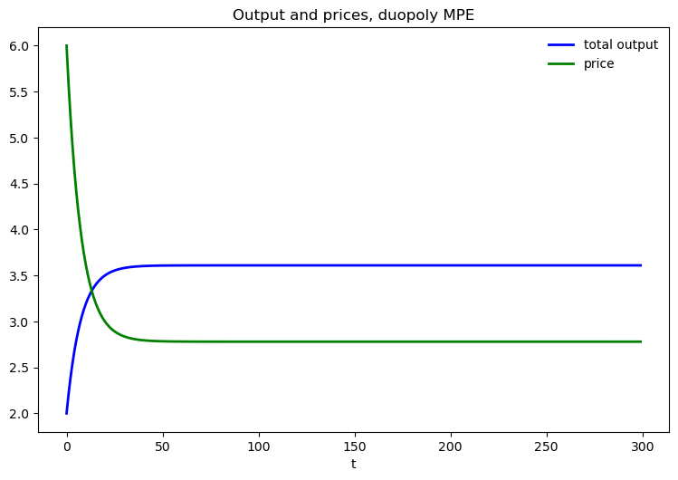
40.12. Markov Perfect Equilibrium#

The state vector is

\[ z_t = \begin{bmatrix} 1 \cr q_{2t} \cr q_{1t} \end{bmatrix} \]

and the state transition dynamics are

\[ z_{t+1} = A z_t + B_1 v_{1t} + B_2 v_{2t} \]

where \(A\) is a \(3 \times 3\) identity matrix and

\[ B_1 = \begin{bmatrix} 0 \cr 0 \cr 1 \end{bmatrix} , \quad B_2 = \begin{bmatrix} 0 \cr 1 \cr 0 \end{bmatrix} \]

The Markov perfect decision rules are

\[ v_{1t} = - F_1 z_t , \quad v_{2t} = - F_2 z_t \]

and in the Markov perfect equilibrium, the state evolves according to

\[ z_{t+1} = (A - B_1 F_1 - B_2 F_2) z_t \]

# In LQ form
A = np.eye(3)
B1 = np.array([[0], [0], [1]])
B2 = np.array([[0], [1], [0]])

R1 = np.array([[0,            0, -a0 / 2],
               [0,            0,  a1 / 2],
               [-a0 / 2, a1 / 2,      a1]])

R2 = np.array([[0,       -a0 / 2,      0],
               [-a0 / 2,      a1, a1 / 2],
               [0,        a1 / 2,      0]])

Q1 = Q2 = γ
S1 = S2 = W1 = W2 = M1 = M2 = 0.0

# Solve using QE's nnash function
F1, F2, P1, P2 = qe.nnash(A, B1, B2, R1, R2, Q1,
                          Q2, S1, S2, W1, W2, M1,
                          M2, beta=β, tol=tol1)

# Simulate forward
AF = A - B1 @ F1 - B2 @ F2
z = np.empty((3, n))
z[:, 0] = 1, 1, 1
for t in range(n-1):
    z[:, t+1] = AF @ z[:, t]

# Display policies
print("Computed policies for firm 1 and firm 2:\n")
print(f"F1 = {F1}")
print(f"F2 = {F2}")

Computed policies for firm 1 and firm 2:

F1 = [[-0.22701363  0.03129874  0.09447113]]
F2 = [[-0.22701363  0.09447113  0.03129874]]

q1 = z[1, :]
q2 = z[2, :]
q = q1 + q2       # Total output, MPE
p = a0 - a1 * q   # Price, MPE

fig, ax = plt.subplots(figsize=(9, 5.8))
ax.plot(range(n), q, 'b-', lw=2, label='total output')
ax.plot(range(n), p, 'g-', lw=2, label='price')
ax.set_title('Output and prices, duopoly MPE')
ax.legend(frameon=False)
ax.set_xlabel('t')
plt.show()

_images/56f2f36fcfe7ed3d030252a73ba09d8e0f5e5060abf8d1a9b6ec9e2cfbbc2ade.png

# Computes the maximum difference between the two quantities of the two firms
np.max(np.abs(q1 - q2))

8.881784197001252e-16

# Compute values
u1 = (- F1 @ z).flatten()
u2 = (- F2 @ z).flatten()

π_1 = p * q1 - γ * (u1) ** 2
π_2 = p * q2 - γ * (u2) ** 2

v1_forward = np.sum(βs * π_1)
v2_forward = np.sum(βs * π_2)

v1_direct = (- z[:, 0].T @ P1 @ z[:, 0])
v2_direct = (- z[:, 0].T @ P2 @ z[:, 0])

# Display values
print("Computed values for firm 1 and firm 2:\n")
print(f"v1(forward sim) = {v1_forward:.4f}; v1 (direct) = {v1_direct:.4f}")
print(f"v2 (forward sim) = {v2_forward:.4f}; v2 (direct) = {v2_direct:.4f}")

Computed values for firm 1 and firm 2:

v1(forward sim) = 133.3303; v1 (direct) = 133.3296
v2 (forward sim) = 133.3303; v2 (direct) = 133.3296

# Sanity check
Λ1 = A - B2 @ F2
lq1 = qe.LQ(Q1, R1, Λ1, B1, beta=β)
P1_ih, F1_ih, d = lq1.stationary_values()

v2_direct_alt = - z[:, 0].T @ lq1.P @ z[:, 0] + lq1.d

(np.abs(v2_direct - v2_direct_alt) < tol2).all()

True

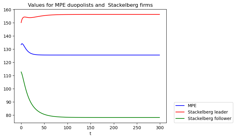
40.13. Comparing Markov Perfect Equilibrium and Stackelberg Outcome#

It is enlightening to compare equilbrium values for firms 1 and 2 under two alternative settings:

A Markov perfect equilibrium like that described in this lecture
A Stackelberg equilbrium

The following code performs the required computations, then plots the continuation values.

vt_MPE = np.zeros(n)
vt_follower = np.zeros(n)

for t in range(n):
    vt_MPE[t] = -z[:, t].T @ P1 @ z[:, t]
    vt_follower[t] = -yt_tilde[:, t].T @ P_tilde @ yt_tilde[:, t]

fig, ax = plt.subplots()
ax.plot(vt_MPE, 'b', label='MPE')
ax.plot(vt_leader, 'r', label='Stackelberg leader')
ax.plot(vt_follower, 'g', label='Stackelberg follower')
ax.set_title(r'Values for MPE duopolists and  Stackelberg firms')
ax.set_xlabel('t')
ax.legend(loc=(1.05, 0))
plt.show()

_images/a64c71a1ac859eea5f8824d05c5ef0dd16822c07172b8dc8541ae4425eafa65a.png

# Display values
print("Computed values:\n")
print(f"vt_leader(y0) = {vt_leader[0]:.4f}")
print(f"vt_follower(y0) = {vt_follower[0]:.4f}")
print(f"vt_MPE(y0) = {vt_MPE[0]:.4f}")

Computed values:

vt_leader(y0) = 150.0324
vt_follower(y0) = 112.6559
vt_MPE(y0) = 133.3296

# Compute the difference in total value between the Stackelberg and the MPE
vt_leader[0] + vt_follower[0] - 2 * vt_MPE[0]

-3.9709425620890784