35. Classical Control with Linear Algebra#
35.1. Overview#
In an earlier lecture Linear Quadratic Dynamic Programming Problems, we have studied how to solve a special class of dynamic optimization and prediction problems by applying the method of dynamic programming. In this class of problems
the objective function is quadratic in states and controls.
the one-step transition function is linear.
shocks are IID Gaussian or martingale differences.
In this lecture and a companion lecture Classical Filtering with Linear Algebra, we study the classical theory of linear-quadratic (LQ) optimal control problems.
The classical approach does not use the two closely related methods – dynamic programming and Kalman filtering – that we describe in other lectures, namely, Linear Quadratic Dynamic Programming Problems and A First Look at the Kalman Filter.
Instead, they use either
\(z\)-transform and lag operator methods, or
matrix decompositions applied to linear systems of first-order conditions for optimum problems.
In this lecture and the sequel Classical Filtering with Linear Algebra, we mostly rely on elementary linear algebra.
The main tool from linear algebra we’ll put to work here is LU decomposition.
We’ll begin with discrete horizon problems.
Then we’ll view infinite horizon problems as appropriate limits of these finite horizon problems.
Later, we will examine the close connection between LQ control and least-squares prediction and filtering problems.
These classes of problems are connected in the sense that to solve each, essentially the same mathematics is used.
Let’s start with some standard imports:
import numpy as np
import matplotlib.pyplot as plt
35.1.1. References#
Useful references include [Whittle, 1963], [Hansen and Sargent, 1980], [Orfanidis, 1988], [Athanasios and Pillai, 1991], and [Muth, 1960].
35.2. A control problem#
Let \(L\) be the lag operator, so that, for sequence \(\{x_t\}\) we have \(L x_t = x_{t-1}\).
More generally, let \(L^k x_t = x_{t-k}\) with \(L^0 x_t = x_t\) and
where \(d_0, d_1, \ldots, d_m\) is a given scalar sequence.
Consider the discrete-time control problem
where
\(h\) is a positive parameter and \(\beta \in (0,1)\) is a discount factor.
\(\{a_t\}_{t \geq 0}\) is a sequence of exponential order less than \(\beta^{-1/2}\), by which we mean \(\lim_{t \rightarrow \infty} \beta^{\frac{t}{2}} a_t = 0\).
Maximization in (35.1) is subject to initial conditions for \(y_{-1}, y_{-2} \ldots, y_{-m}\).
Maximization is over infinite sequences \(\{y_t\}_{t \geq 0}\).
35.2.1. Example#
The formulation of the LQ problem given above is broad enough to encompass many useful models.
As a simple illustration, recall that in LQ Control: Foundations we consider a monopolist facing stochastic demand shocks and adjustment costs.
Let’s consider a deterministic version of this problem, where the monopolist maximizes the discounted sum
and
In this expression, \(q_t\) is output, \(c\) is average cost of production, and \(d_t\) is a demand shock.
The term \(\gamma (q_{t+1} - q_t)^2\) represents adjustment costs.
You will be able to confirm that the objective function can be rewritten as (35.1) when
\(a_t := \alpha_0 + d_t - c\)
\(h := 2 \alpha_1\)
\(d(L) := \sqrt{2 \gamma}(I - L)\)
Further examples of this problem for factor demand, economic growth, and government policy problems are given in ch. IX of [Sargent, 1987].
35.3. Finite horizon theory#
We first study a finite \(N\) version of the problem.
Later we will study an infinite horizon problem solution as a limiting version of a finite horizon problem.
(This will require being careful because the limits as \(N \to \infty\) of the necessary and sufficient conditions for maximizing finite \(N\) versions of (35.1) are not sufficient for maximizing (35.1))
We begin by
fixing \(N > m\),
differentiating the finite version of (35.1) with respect to \(y_0, y_1, \ldots, y_N\), and
setting these derivatives to zero.
For \(t=0, \ldots, N-m\) these first-order necessary conditions are the Euler equations.
For \(t = N-m + 1, \ldots, N\), the first-order conditions are a set of terminal conditions.
Consider the term
Differentiating \(J\) with respect to \(y_t\) for \(t=0,\ 1,\ \ldots,\ N-m\) gives
We can write this more succinctly as
Differentiating \(J\) with respect to \(y_t\) for \(t = N-m + 1, \ldots, N\) gives
With these preliminaries under our belts, we are ready to differentiate (35.1).
Differentiating (35.1) with respect to \(y_t\) for \(t=0, \ldots, N-m\) gives the Euler equations
The system of equations (35.4) forms a \(2 \times m\) order linear difference equation that must hold for the values of \(t\) indicated.
Differentiating (35.1) with respect to \(y_t\) for \(t = N-m + 1, \ldots, N\) gives the terminal conditions
In the finite \(N\) problem, we want simultaneously to solve (35.4) subject to the \(m\) initial conditions \(y_{-1}, \ldots, y_{-m}\) and the \(m\) terminal conditions (35.5).
These conditions uniquely pin down the solution of the finite \(N\) problem.
That is, for the finite \(N\) problem, conditions (35.4) and (35.5) are necessary and sufficient for a maximum, by concavity of the objective function.
Next, we describe how to obtain the solution using matrix methods.
35.3.1. Matrix methods#
Let’s look at how linear algebra can be used to tackle and shed light on the finite horizon LQ control problem.
35.3.1.1. A single lag term#
Let’s begin with the special case in which \(m=1\).
We want to solve the system of \(N+1\) linear equations
where \(d(L) = d_0 + d_1 L\).
These equations are to be solved for \(y_0, y_1, \ldots, y_N\) as functions of \(a_0, a_1, \ldots, a_N\) and \(y_{-1}\).
Let
Then we can represent (35.6) as the matrix equation
or
Notice how we have chosen to arrange the \(y_t\)’s in reverse time order.
The matrix \(W\) on the left side of (35.7) is “almost” a Toeplitz matrix (where each descending diagonal is constant).
There are two sources of deviation from the form of a Toeplitz matrix
The first element differs from the remaining diagonal elements, reflecting the terminal condition.
The sub-diagonal elements equal \(\beta\) time the super-diagonal elements.
The solution of (35.8) can be expressed in the form
which represents each element \(y_t\) of \(\bar y\) as a function of the entire vector \(\bar a\).
That is, \(y_t\) is a function of past, present, and future values of \(a\)’s, as well as of the initial condition \(y_{-1}\).
35.3.1.2. An alternative representation#
An alternative way to express the solution to (35.7) or (35.8) is in so-called feedback-feedforward form.
The idea here is to find a solution expressing \(y_t\) as a function of past \(y\)’s and current and future \(a\)’s.
To achieve this solution, one can use an LU decomposition of \(W\).
There always exists a decomposition of \(W\) of the form \(W= LU\) where
\(L\) is an \((N+1) \times (N+1)\) lower triangular matrix.
\(U\) is an \((N+1) \times (N+1)\) upper triangular matrix.
The factorization can be normalized so that the diagonal elements of \(U\) are unity.
Using the LU representation in (35.9), we obtain
Since \(L^{-1}\) is lower triangular, this representation expresses \(y_t\) as a function of
lagged \(y\)’s (via the term \(U \bar y\)), and
current and future \(a\)’s (via the term \(L^{-1} \bar a\))
Because there are zeros everywhere in the matrix on the left of (35.7) except on the diagonal, super-diagonal, and sub-diagonal, the \(LU\) decomposition takes
\(L\) to be zero except in the diagonal and the leading sub-diagonal.
\(U\) to be zero except on the diagonal and the super-diagonal.
Thus, (35.10) has the form
where \(L^{-1}_{ij}\) is the \((i,j)\) element of \(L^{-1}\) and \(U_{ij}\) is the \((i,j)\) element of \(U\).
Note how the left side for a given \(t\) involves \(y_t\) and one lagged value \(y_{t-1}\) while the right side involves all future values of the forcing process \(a_t, a_{t+1}, \ldots, a_N\).
35.3.1.3. Additional lag terms#
We briefly indicate how this approach extends to the problem with \(m > 1\).
Assume that \(\beta = 1\) and let \(D_{m+1}\) be the \((m+1) \times (m+1)\) symmetric matrix whose elements are determined from the following formula:
Let \(I_{m+1}\) be the \((m+1) \times (m+1)\) identity matrix.
Let \(\phi_j\) be the coefficients in the expansion \(\phi (L) = h + d (L^{-1}) d (L)\).
Then the first order conditions (35.4) and (35.5) can be expressed as:
where \(M\) is \((m+1)\times m\) and
As before, we can express this equation as \(W \bar y = \bar a\).
The matrix on the left of this equation is “almost” Toeplitz, the exception being the leading \(m \times m\) submatrix in the upper left-hand corner.
We can represent the solution in feedback-feedforward form by obtaining a decomposition \(LU = W\), and obtain
where \(L^{-1}_{t,s}\) is the element in the \((t,s)\) position of \(L\), and similarly for \(U\).
The left side of equation (35.11) is the “feedback” part of the optimal control law for \(y_t\), while the right-hand side is the “feedforward” part.
We note that there is a different control law for each \(t\).
Thus, in the finite horizon case, the optimal control law is time-dependent.
It is natural to suspect that as \(N \rightarrow\infty\), (35.11) becomes equivalent to the solution of our infinite horizon problem, which below we shall show can be expressed as
so that as \(N \rightarrow \infty\) we expect that for each fixed \(t, U^{-1}_{t, t-j} \rightarrow c_j\) and \(L_{t,t+j}\) approaches the coefficient on \(L^{-j}\) in the expansion of \(c(\beta L^{-1})^{-1}\).
This suspicion is true under general conditions that we shall study later.
For now, we note that by creating the matrix \(W\) for large \(N\) and factoring it into the \(LU\) form, good approximations to \(c(L)\) and \(c(\beta L^{-1})^{-1}\) can be obtained.
35.4. Infinite horizon limit#
For the infinite horizon problem, we propose to discover first-order necessary conditions by taking the limits of (35.4) and (35.5) as \(N \to \infty\).
This approach is valid, and the limits of (35.4) and (35.5) as \(N\) approaches infinity are first-order necessary conditions for a maximum.
However, for the infinite horizon problem with \(\beta < 1\), the limits of (35.4) and (35.5) are, in general, not sufficient for a maximum.
That is, the limits of (35.5) do not provide enough information uniquely to determine the solution of the Euler equation (35.4) that maximizes (35.1).
As we shall see below, a side condition on the path of \(y_t\) that together with (35.4) is sufficient for an optimum is
All paths that satisfy the Euler equations, except the one that we shall select below, violate this condition and, therefore, evidently lead to (much) lower values of (35.1) than does the optimal path selected by the solution procedure below.
Consider the characteristic equation associated with the Euler equation
Notice that if \(\tilde z\) is a root of equation (35.13), then so is \(\beta \tilde z^{-1}\).
Thus, the roots of (35.13) come in “\(\beta\)-reciprocal” pairs.
Assume that the roots of (35.13) are distinct.
Let the roots be, in descending order according to their moduli, \(z_1, z_2, \ldots, z_{2m}\).
From the reciprocal pairs property and the assumption of distinct roots, it follows that \(\vert z_j \vert > \sqrt \beta\ \hbox{ for } j\leq m \hbox { and } \vert z_j \vert < \sqrt\beta\ \hbox { for } j > m\).
It also follows that \(z_{2m-j} = \beta z^{-1}_{j+1}, j=0, 1, \ldots, m-1\).
Therefore, the characteristic polynomial on the left side of (35.13) can be expressed as
where \(z_0\) is a constant.
In (35.14), we substitute \((z-z_j) = -z_j (1- {1 \over z_j}z)\) and \((z-\beta z_j^{-1}) = z(1 - {\beta \over z_j} z^{-1})\) for \(j = 1, \ldots, m\) to get
Now define \(c(z) = \sum^m_{j=0} c_j \, z^j\) as
Notice that (35.14) can be written
It is useful to write (35.15) as
where
Since \(\vert z_j \vert > \sqrt \beta \hbox { for } j = 1, \ldots, m\) it follows that \(\vert \lambda_j \vert < 1/\sqrt \beta\) for \(j = 1, \ldots, m\).
Using (35.17), we can express the factorization (35.16) as
In sum, we have constructed a factorization (35.16) of the characteristic polynomial for the Euler equation in which the zeros of \(c(z)\) exceed \(\beta^{1/2}\) in modulus, and the zeros of \(c\,(\beta z^{-1})\) are less than \(\beta^{1/2}\) in modulus.
Using (35.16), we now write the Euler equation as
The unique solution of the Euler equation that satisfies condition (35.12) is
This can be established by using an argument paralleling that in chapter IX of [Sargent, 1987].
To exhibit the solution in a form paralleling that of [Sargent, 1987], we use (35.17) to write (35.18) as
Using partial fractions, we can write the characteristic polynomial on the right side of (35.19) as
Then (35.19) can be written
or
Equation (35.20) expresses the optimum sequence for \(y_t\) in terms of \(m\) lagged \(y\)’s, and \(m\) weighted infinite geometric sums of future \(a_t\)’s.
Furthermore, (35.20) is the unique solution of the Euler equation that satisfies the initial conditions and condition (35.12).
In effect, condition (35.12) compels us to solve the “unstable” roots of \(h+d (\beta z^{-1})d(z)\) forward (see [Sargent, 1987]).
The step of factoring the polynomial \(h+d (\beta z^{-1})\, d(z)\) into \(c\, (\beta z^{-1})c\,(z)\), where the zeros of \(c\,(z)\) all have modulus exceeding \(\sqrt\beta\), is central to solving the problem.
We note two features of the solution (35.20)
Since \(\vert \lambda_j \vert < 1/\sqrt \beta\) for all \(j\), it follows that \((\lambda_j \ \beta) < \sqrt \beta\).
The assumption that \(\{ a_t \}\) is of exponential order less than \(1 /\sqrt \beta\) is sufficient to guarantee that the geometric sums of future \(a_t\)’s on the right side of (35.20) converge.
We immediately see that those sums will converge under the weaker condition that \(\{ a_t\}\) is of exponential order less than \(\phi^{-1}\) where \(\phi = \max \, \{\beta \lambda_i, i=1,\ldots,m\}\).
Note that with \(a_t\) identically zero, (35.20) implies that in general \(\vert y_t \vert\) eventually grows exponentially at a rate given by \(\max_i \vert \lambda_i \vert\).
The condition \(\max_i \vert \lambda_i \vert <1 /\sqrt \beta\) guarantees that condition (35.12) is satisfied.
In fact, \(\max_i \vert \lambda_i \vert < 1 /\sqrt \beta\) is a necessary condition for (35.12) to hold.
Were (35.12) not satisfied, the objective function would diverge to \(- \infty\), implying that the \(y_t\) path could not be optimal.
For example, with \(a_t = 0\), for all \(t\), it is easy to describe a naive (nonoptimal) policy for \(\{y_t, t\geq 0\}\) that gives a finite value of (35.17).
We can simply let \(y_t = 0 \hbox { for } t\geq 0\).
This policy involves at most \(m\) nonzero values of \(hy^2_t\) and \([d(L)y_t]^2\), and so yields a finite value of (35.1).
Therefore it is easy to dominate a path that violates (35.12).
35.5. Undiscounted problems#
It is worthwhile focusing on a special case of the LQ problems above: the undiscounted problem that emerges when \(\beta = 1\).
In this case, the Euler equation is
The factorization of the characteristic polynomial (35.16) becomes
where
The solution of the problem becomes
35.5.1. Transforming discounted to undiscounted problem#
Discounted problems can always be converted into undiscounted problems via a simple transformation.
Consider problem (35.1) with \(0 < \beta < 1\).
Define the transformed variables
Then notice that \(\beta^t\,[d\, (L) y_t ]^2=[\tilde d\,(L)\tilde y_t]^2\) with \(\tilde d \,(L)=\sum^m_{j=0} \tilde d_j\, L^j\) and \(\tilde d_j = \beta^{j/2} d_j\).
Then the original criterion function (35.1) is equivalent to
which is to be maximized over sequences \(\{\tilde y_t,\ t=0, \ldots\}\) subject to \(\tilde y_{-1}, \cdots, \tilde y_{-m}\) given and \(\{\tilde a_t,\ t=1, \ldots\}\) a known bounded sequence.
The Euler equation for this problem is \([h+\tilde d \,(L^{-1}) \, \tilde d\, (L) ]\, \tilde y_t = \tilde a_t\).
The solution is
or
where \(\tilde c \,(z^{-1}) \tilde c\,(z) = h + \tilde d\,(z^{-1}) \tilde d \,(z)\), and where
We leave it to the reader to show that (35.23) implies the equivalent form of the solution
where
The transformations (35.21) and the inverse formulas (35.24) allow us to solve a discounted problem by first solving a related undiscounted problem.
35.6. Implementation#
Here’s the code that computes solutions to the LQ problem using the methods described above.
import numpy as np
import scipy.stats as spst
import scipy.linalg as la

class LQFilter:

    def __init__(self, d, h, y_m, r=None, h_eps=None, β=None):
        """

        Parameters
        ----------
            d : list or numpy.array (1-D or a 2-D column vector)
                    The order of the coefficients: [d_0, d_1, ..., d_m]
            h : scalar
                    Parameter of the objective function (corresponding to the
                    quadratic term)
            y_m : list or numpy.array (1-D or a 2-D column vector)
                    Initial conditions for y
            r : list or numpy.array (1-D or a 2-D column vector)
                    The order of the coefficients: [r_0, r_1, ..., r_k]
                    (optional, if not defined -> deterministic problem)
            β : scalar
                    Discount factor (optional, default value is one)
        """

        self.h = h
        self.d = np.asarray(d)
        self.m = self.d.shape[0] - 1

        self.y_m = np.asarray(y_m)

        if self.m == self.y_m.shape[0]:
            self.y_m = self.y_m.reshape(self.m, 1)
        else:
            raise ValueError("y_m must be of length m = {self.m:d}")

        #---------------------------------------------
        # Define the coefficients of ϕ upfront
        #---------------------------------------------
        ϕ = np.zeros(2 * self.m + 1)
        for i in range(- self.m, self.m + 1):
            ϕ[self.m - i] = np.sum(np.diag(self.d.reshape(self.m + 1, 1) \
                                           @ self.d.reshape(1, self.m + 1),
                                           k=-i
                                           )
                                    )
        ϕ[self.m] = ϕ[self.m] + self.h
        self.ϕ = ϕ

        #-----------------------------------------------------
        # If r is given calculate the vector ϕ_r
        #-----------------------------------------------------
        if r is None:
            pass
        else:
            self.r = np.asarray(r)
            self.k = self.r.shape[0] - 1
            ϕ_r = np.zeros(2 * self.k + 1)
            for i in range(- self.k, self.k + 1):
                ϕ_r[self.k - i] = np.sum(np.diag(self.r.reshape(self.k + 1, 1) \
                                                 @ self.r.reshape(1, self.k + 1),
                                                 k=-i
                                                 )
                                        )
            if h_eps is None:
                self.ϕ_r = ϕ_r
            else:
                ϕ_r[self.k] = ϕ_r[self.k] + h_eps
                self.ϕ_r = ϕ_r

        #-----------------------------------------------------
        # If β is given, define the transformed variables
        #-----------------------------------------------------
        if β is None:
            self.β = 1
        else:
            self.β = β
            self.d = self.β**(np.arange(self.m + 1)/2) * self.d
            self.y_m = self.y_m * (self.β**(- np.arange(1, self.m + 1)/2)) \
                                   .reshape(self.m, 1)

    def construct_W_and_Wm(self, N):
        """
        This constructs the matrices W and W_m for a given number of periods N
        """

        m = self.m
        d = self.d

        W = np.zeros((N + 1, N + 1))
        W_m = np.zeros((N + 1, m))

        #---------------------------------------
        # Terminal conditions
        #---------------------------------------

        D_m1 = np.zeros((m + 1, m + 1))
        M = np.zeros((m + 1, m))

        # (1) Constuct the D_{m+1} matrix using the formula

        for j in range(m + 1):
            for k in range(j, m + 1):
                D_m1[j, k] = d[:j + 1] @ d[k - j: k + 1]

        # Make the matrix symmetric
        D_m1 = D_m1 + D_m1.T - np.diag(np.diag(D_m1))

        # (2) Construct the M matrix using the entries of D_m1

        for j in range(m):
            for i in range(j + 1, m + 1):
                M[i, j] = D_m1[i - j - 1, m]

        #----------------------------------------------
        # Euler equations for t = 0, 1, ..., N-(m+1)
        #----------------------------------------------
        ϕ = self.ϕ

        W[:(m + 1), :(m + 1)] = D_m1 + self.h * np.eye(m + 1)
        W[:(m + 1), (m + 1):(2 * m + 1)] = M

        for i, row in enumerate(np.arange(m + 1, N + 1 - m)):
            W[row, (i + 1):(2 * m + 2 + i)] = ϕ

        for i in range(1, m + 1):
            W[N - m + i, -(2 * m + 1 - i):] = ϕ[:-i]

        for i in range(m):
            W_m[N - i, :(m - i)] = ϕ[(m + 1 + i):]

        return W, W_m

    def roots_of_characteristic(self):
        """
        This function calculates z_0 and the 2m roots of the characteristic
        equation associated with the Euler equation (1.7)

        Note:
        ------
        numpy.poly1d(roots, True) defines a polynomial using its roots that can
        be evaluated at any point. If x_1, x_2, ... , x_m are the roots then
            p(x) = (x - x_1)(x - x_2)...(x - x_m)
        """
        m = self.m
        ϕ = self.ϕ

        # Calculate the roots of the 2m-polynomial
        roots = np.roots(ϕ)
        # Sort the roots according to their length (in descending order)
        roots_sorted = roots[np.argsort(abs(roots))[::-1]]

        z_0 = ϕ.sum() / np.poly1d(roots, True)(1)
        z_1_to_m = roots_sorted[:m]     # We need only those outside the unit circle

        λ = 1 / z_1_to_m

        return z_1_to_m, z_0, λ

    def coeffs_of_c(self):
        '''
        This function computes the coefficients {c_j, j = 0, 1, ..., m} for
                c(z) = sum_{j = 0}^{m} c_j z^j

        Based on the expression (1.9). The order is
            c_coeffs = [c_0, c_1, ..., c_{m-1}, c_m]
        '''
        z_1_to_m, z_0 = self.roots_of_characteristic()[:2]

        c_0 = (z_0 * np.prod(z_1_to_m).real * (- 1)**self.m)**(.5)
        c_coeffs = np.poly1d(z_1_to_m, True).c * z_0 / c_0

        return c_coeffs[::-1]

    def solution(self):
        """
        This function calculates {λ_j, j=1,...,m} and {A_j, j=1,...,m}
        of the expression (1.15)
        """
        λ = self.roots_of_characteristic()[2]
        c_0 = self.coeffs_of_c()[-1]

        A = np.zeros(self.m, dtype=complex)
        for j in range(self.m):
            denom = 1 - λ/λ[j]
            A[j] = c_0**(-2) / np.prod(denom[np.arange(self.m) != j])

        return λ, A

    def construct_V(self, N):
        '''
        This function constructs the covariance matrix for x^N (see section 6)
        for a given period N
        '''
        V = np.zeros((N, N))
        ϕ_r = self.ϕ_r

        for i in range(N):
            for j in range(N):
                if abs(i-j) <= self.k:
                    V[i, j] = ϕ_r[self.k + abs(i-j)]

        return V

    def simulate_a(self, N):
        """
        Assuming that the u's are normal, this method draws a random path
        for x^N
        """
        V = self.construct_V(N + 1)
        d = spst.multivariate_normal(np.zeros(N + 1), V)

        return d.rvs()

    def predict(self, a_hist, t):
        """
        This function implements the prediction formula discussed in section 6 (1.59)
        It takes a realization for a^N, and the period in which the prediction is
        formed

        Output:  E[abar | a_t, a_{t-1}, ..., a_1, a_0]
        """

        N = np.asarray(a_hist).shape[0] - 1
        a_hist = np.asarray(a_hist).reshape(N + 1, 1)
        V = self.construct_V(N + 1)

        aux_matrix = np.zeros((N + 1, N + 1))
        aux_matrix[:(t + 1), :(t + 1)] = np.eye(t + 1)
        L = la.cholesky(V).T
        Ea_hist = la.inv(L) @ aux_matrix @ L @ a_hist

        return Ea_hist

    def optimal_y(self, a_hist, t=None):
        """
        - if t is NOT given it takes a_hist (list or numpy.array) as a
          deterministic a_t
        - if t is given, it solves the combined control prediction problem
          (section 7)(by default, t == None -> deterministic)

        for a given sequence of a_t (either deterministic or a particular
        realization), it calculates the optimal y_t sequence using the method
        of the lecture

        Note:
        ------
        scipy.linalg.lu normalizes L, U so that L has unit diagonal elements
        To make things consistent with the lecture, we need an auxiliary
        diagonal matrix D which renormalizes L and U
        """

        N = np.asarray(a_hist).shape[0] - 1
        W, W_m = self.construct_W_and_Wm(N)

        L, U = la.lu(W, permute_l=True)
        D = np.diag(1 / np.diag(U))
        U = D @ U
        L = L @ np.diag(1 / np.diag(D))

        J = np.fliplr(np.eye(N + 1))

        if t is None:   # If the problem is deterministic

            a_hist = J @ np.asarray(a_hist).reshape(N + 1, 1)

            #--------------------------------------------
            # Transform the 'a' sequence if β is given
            #--------------------------------------------
            if self.β != 1:
                a_hist =  a_hist * (self.β**(np.arange(N + 1) / 2))[::-1] \
                                    .reshape(N + 1, 1)

            a_bar = a_hist - W_m @ self.y_m            # a_bar from the lecture
            Uy = np.linalg.solve(L, a_bar)             # U @ y_bar = L^{-1}
            y_bar = np.linalg.solve(U, Uy)             # y_bar = U^{-1}L^{-1}

            # Reverse the order of y_bar with the matrix J
            J = np.fliplr(np.eye(N + self.m + 1))
            # y_hist : concatenated y_m and y_bar
            y_hist = J @ np.vstack([y_bar, self.y_m])

            #--------------------------------------------
            # Transform the optimal sequence back if β is given
            #--------------------------------------------
            if self.β != 1:
                y_hist = y_hist * (self.β**(- np.arange(-self.m, N + 1)/2)) \
                                    .reshape(N + 1 + self.m, 1)

            return y_hist, L, U, y_bar

        else:           # If the problem is stochastic and we look at it

            Ea_hist = self.predict(a_hist, t).reshape(N + 1, 1)
            Ea_hist = J @ Ea_hist

            a_bar = Ea_hist - W_m @ self.y_m           # a_bar from the lecture
            Uy = np.linalg.solve(L, a_bar)             # U @ y_bar = L^{-1}
            y_bar = np.linalg.solve(U, Uy)             # y_bar = U^{-1}L^{-1}

            # Reverse the order of y_bar with the matrix J
            J = np.fliplr(np.eye(N + self.m + 1))
            # y_hist : concatenated y_m and y_bar
            y_hist = J @ np.vstack([y_bar, self.y_m])

            return y_hist, L, U, y_bar
35.6.1. Example#
In this application, we’ll have one lag, with
Suppose for the moment that \(\gamma = 0\).
Then the intertemporal component of the LQ problem disappears, and the agent simply wants to maximize \(a_t y_t - hy^2_t / 2\) in each period.
This means that the agent chooses \(y_t = a_t / h\).
In the following we’ll set \(h = 1\), so that the agent just wants to track the \(\{a_t\}\) process.
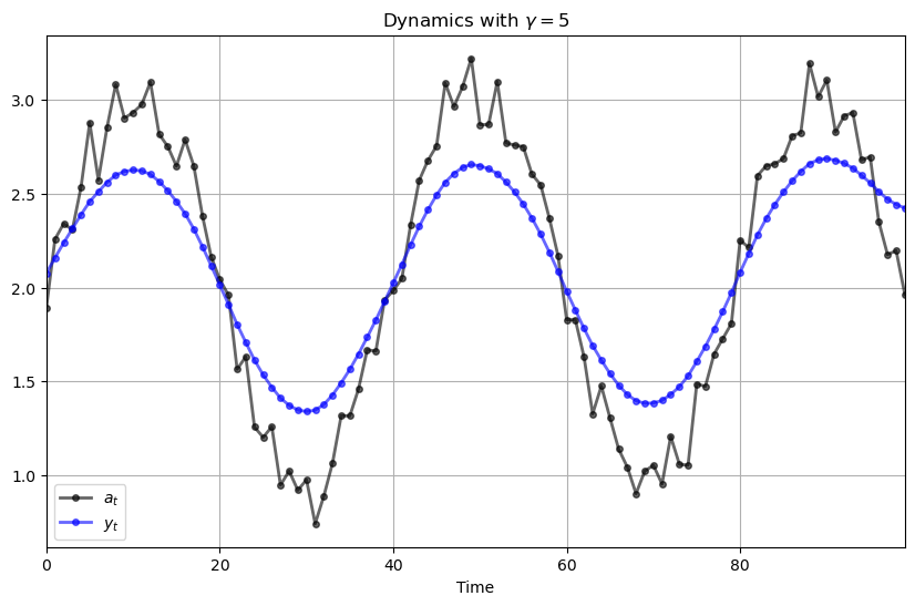
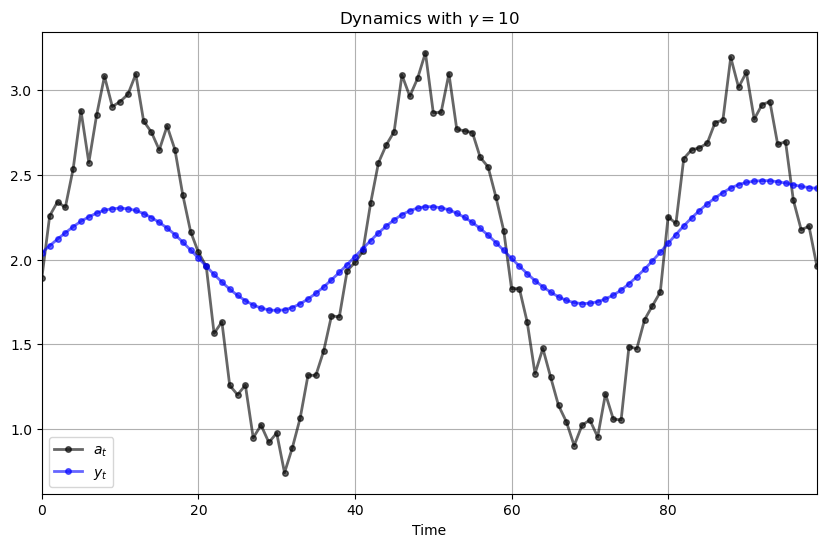
However, as we increase \(\gamma\), the agent gives greater weight to a smooth time path.
Hence \(\{y_t\}\) evolves as a smoothed version of \(\{a_t\}\).
The \(\{a_t\}\) sequence we’ll choose as a stationary cyclic process plus some white noise.
Here’s some code that generates a plot when \(\gamma = 0.8\)
# Set seed and generate a_t sequence
np.random.seed(123)
n = 100
a_seq = np.sin(np.linspace(0, 5 * np.pi, n)) + 2 + 0.1 * np.random.randn(n)

def plot_simulation(γ=0.8, m=1, h=1, y_m=2):

    d = γ * np.asarray([1, -1])
    y_m = np.asarray(y_m).reshape(m, 1)

    testlq = LQFilter(d, h, y_m)
    y_hist, L, U, y = testlq.optimal_y(a_seq)
    y = y[::-1]  # Reverse y

    # Plot simulation results

    fig, ax = plt.subplots(figsize=(10, 6))
    p_args = {'lw' : 2, 'alpha' : 0.6}
    time = range(len(y))
    ax.plot(time, a_seq / h, 'k-o', ms=4, lw=2, alpha=0.6, label='$a_t$')
    ax.plot(time, y, 'b-o', ms=4, lw=2, alpha=0.6, label='$y_t$')
    ax.set(title=rf'Dynamics with $\gamma = {γ}$',
           xlabel='Time',
           xlim=(0, max(time))
          )
    ax.legend()
    ax.grid()
    plt.show()

plot_simulation()

Here’s what happens when we change \(\gamma\) to 5.0
plot_simulation(γ=5)
And here’s \(\gamma = 10\)
plot_simulation(γ=10)
35.7. Exercises#
Exercise 35.1
Consider solving a discounted version \((\beta < 1)\) of problem (35.1), as follows.
Convert (35.1) to the undiscounted problem (35.22).
Let the solution of (35.22) in feedback form be
or
Here
\(h + \tilde d (z^{-1}) \tilde d (z) = \tilde c (z^{-1}) \tilde c (z)\)
\(\tilde c (z) = [(-1)^m \tilde z_0 \tilde z_1 \cdots \tilde z_m ]^{1/2} (1 - \tilde \lambda_1 z) \cdots (1 - \tilde \lambda_m z)\)
where the \(\tilde z_j\) are the zeros of \(h +\tilde d (z^{-1})\, \tilde d(z)\).
Prove that (35.25) implies that the solution for \(y_t\) in feedback form is
where \(f_j = \tilde f_j \beta^{-j/2}, A_j = \tilde A_j\), and \(\lambda_j = \tilde \lambda_j \beta^{-1/2}\).
Exercise 35.2
Solve the optimal control problem, maximize
subject to \(y_{-1}\) given, and \(\{ a_t\}\) a known bounded sequence.
Express the solution in the “feedback form” (35.20), giving numerical values for the coefficients.
Make sure that the boundary conditions (35.5) are satisfied.
Note
This problem differs from the problem in the text in one important way: instead of \(h > 0\) in (35.1), \(h = 0\). This has an important influence on the solution.
Exercise 35.3
Solve the infinite time-optimal control problem to maximize
subject to \(y_{-1}\) given. Prove that the solution is
Exercise 35.4
Solve the infinite time problem, to maximize
subject to \(y_{-1}\) given. Prove that the solution \(y_t = 2y_{t-1}\) violates condition (35.12), and so is not optimal.
Prove that the optimal solution is approximately \(y_t = .5 y_{t-1}\).