24. Rosen Schooling Model#

This lecture is yet another part of a suite of lectures that use the quantecon DLE class to instantiate models within the [Hansen and Sargent, 2013] class of models described in detail in Recursive Models of Dynamic Linear Economies.

In addition to what’s included in Anaconda, this lecture uses the quantecon library

!pip install --upgrade quantecon

We’ll also need the following imports:

import numpy as np
import matplotlib.pyplot as plt
from collections import namedtuple
from quantecon import DLE

24.1. A one-occupation model#

Ryoo and Rosen’s (2004) [Ryoo and Rosen, 2004] partial equilibrium model determines

a stock of “Engineers” \(N_t\)
a number of new entrants in engineering school, \(n_t\)
the wage rate of engineers, \(w_t\)

It takes k periods of schooling to become an engineer.

The model consists of the following equations:

a demand curve for engineers:

\[ w_t = - \alpha_d N_t + \epsilon_{dt} \]

a time-to-build structure of the education process:

\[ N_{t+k} = \delta_N N_{t+k-1} + n_t \]

a definition of the discounted present value of each new engineering student:

\[ v_t = \beta^k \mathbb{E} \sum_{j=0}^\infty (\beta \delta_N)^j w_{t+k+j} \]

a supply curve of new students driven by present value \(v_t\):

\[ n_t = \alpha_s v_t + \epsilon_{st} \]

24.2. Mapping into Hansen-Sargent (2013) framework#

We represent this model in the [Hansen and Sargent, 2013] framework by

sweeping the time-to-build structure and the demand for engineers into the household technology, and
putting the supply of engineers into the technology for producing goods

24.2.1. Preferences#

\[\begin{split} \Pi = 0, \Lambda= \begin{bmatrix} \alpha_d & 0 & \cdots & 0 \end{bmatrix} , \Delta_h = \begin{bmatrix} \delta_N & 1 & 0 & \cdots & 0 \\ 0 & 0 & 1 & \cdots & 0 \\ \vdots & \vdots & \vdots & \ddots & \vdots \\ 0 & \cdots& \cdots & 0 & 1 \\ 0 & 0 & 0 & \cdots & 0 \end{bmatrix} , \Theta_h = \begin{bmatrix} 0 \\ 0 \\ \vdots \\ 0 \\ 1 \end{bmatrix} \end{split}\]

where \(\Lambda\) is a \(1 \times (k+1)\) matrix, \(\Delta_h\) is a \((k+1) \times (k+1)\) matrix, and \(\Theta_h\) is a \((k+1) \times 1\) matrix.

This specification sets \(N_t = h_{1t-1}\), \(n_t = c_t\), \(h_{\tau+1,t-1} = n_{t-(k-\tau)}\) for \(\tau = 1,...,k\).

Below we set things up so that the number of years of education, \(k\), can be varied.

24.2.2. Technology#

To capture Ryoo and Rosen’s [Ryoo and Rosen, 2004] supply curve, we use the physical technology:

\[ c_t = i_t + d_{1t} \]

\[ \psi_1i_t = g_t \]

where \(\psi_1\) is inversely proportional to \(\alpha_s\).

24.2.3. Information#

Because we want \(b_t = \epsilon_{dt}\) and \(d_{1t} =\epsilon_{st}\), we set

\[\begin{split} A_{22}= \begin{bmatrix} 1 & 0 & 0 \\ 0 & \rho_s & 0 \\ 0 & 0 & \rho_d \end{bmatrix} , C_2 = \begin{bmatrix} 0 & 0 \\ 1 & 0 \\ 0 & 1 \end{bmatrix} , U_b = \begin{bmatrix} 30 & 0 & 1 \end{bmatrix} , U_d = \begin{bmatrix} 10 & 1 & 0 \\ 0 & 0 & 0 \end{bmatrix} \end{split}\]

where \(\rho_s\) and \(\rho_d\) describe the persistence of the supply and demand shocks

Information = namedtuple('Information', ['a22', 'c2','ub','ud'])
Technology = namedtuple('Technology', ['ϕ_c', 'ϕ_g', 'ϕ_i', 'γ', 'δ_k', 'θ_k'])
Preferences = namedtuple('Preferences', ['β', 'l_λ', 'π_h', 'δ_h', 'θ_h'])

24.2.4. Effects of changes in education technology and demand#

We now study how changing

the number of years of education required to become an engineer and
the slope of the demand curve

affects responses to demand shocks.

To begin, we set \(k = 4\) and \(\alpha_d = 0.1\)

k = 4  # Number of periods of schooling required to become an engineer

β = np.array([[1 / 1.05]])
α_d = np.array([[0.1]])
α_s = 1
ε_1 = 1e-7
λ_1 = np.full((1, k), ε_1)
# Use of ε_1 is a trick to acquire detectability, see HS2013 p. 228 footnote 4
l_λ = np.hstack((α_d, λ_1))
π_h = np.array([[0]])

δ_n = np.array([[0.95]])
d1 = np.vstack((δ_n, np.zeros((k - 1, 1))))
d2 = np.hstack((d1, np.eye(k)))
δ_h = np.vstack((d2, np.zeros((1, k + 1))))

θ_h = np.vstack((np.zeros((k, 1)),
                 np.ones((1, 1))))

ψ_1 = 1 / α_s

ϕ_c = np.array([[1], [0]])
ϕ_g = np.array([[0], [-1]])
ϕ_i = np.array([[-1], [ψ_1]])
γ = np.array([[0], [0]])

δ_k = np.array([[0]])
θ_k = np.array([[0]])

ρ_s = 0.8
ρ_d = 0.8

a22 = np.array([[1,   0,   0],
                [0, ρ_s,   0],
                [0,   0, ρ_d]])

c2 = np.array([[0, 0], [10, 0], [0, 10]])
ub = np.array([[30, 0, 1]])
ud = np.array([[10, 1, 0], [0, 0, 0]])

info1 = Information(a22, c2, ub, ud)
tech1 = Technology(ϕ_c, ϕ_g, ϕ_i, γ, δ_k, θ_k)
pref1 = Preferences(β, l_λ, π_h, δ_h, θ_h)

econ1 = DLE(info1, tech1, pref1)

We create three other instances by:

Raising \(\alpha_d\) to 2
Raising \(k\) to 7
Raising \(k\) to 10

α_d = np.array([[2]])
l_λ = np.hstack((α_d, λ_1))
pref2 = Preferences(β, l_λ, π_h, δ_h, θ_h)
econ2 = DLE(info1, tech1, pref2)

α_d = np.array([[0.1]])

k = 7
λ_1 = np.full((1, k), ε_1)
l_λ = np.hstack((α_d, λ_1))
d1 = np.vstack((δ_n, np.zeros((k - 1, 1))))
d2 = np.hstack((d1, np.eye(k)))
δ_h = np.vstack((d2, np.zeros((1, k+1))))
θ_h = np.vstack((np.zeros((k, 1)),
                 np.ones((1, 1))))

Pref3 = Preferences(β, l_λ, π_h, δ_h, θ_h)
econ3 = DLE(info1, tech1, Pref3)

k = 10
λ_1 = np.full((1, k), ε_1)
l_λ = np.hstack((α_d, λ_1))
d1 = np.vstack((δ_n, np.zeros((k - 1, 1))))
d2 = np.hstack((d1, np.eye(k)))
δ_h = np.vstack((d2, np.zeros((1, k + 1))))
θ_h = np.vstack((np.zeros((k, 1)),
                 np.ones((1, 1))))

pref4 = Preferences(β, l_λ, π_h, δ_h, θ_h)
econ4 = DLE(info1, tech1, pref4)

shock_demand = np.array([[0], [1]])

econ1.irf(ts_length=25, shock=shock_demand)
econ2.irf(ts_length=25, shock=shock_demand)
econ3.irf(ts_length=25, shock=shock_demand)
econ4.irf(ts_length=25, shock=shock_demand)

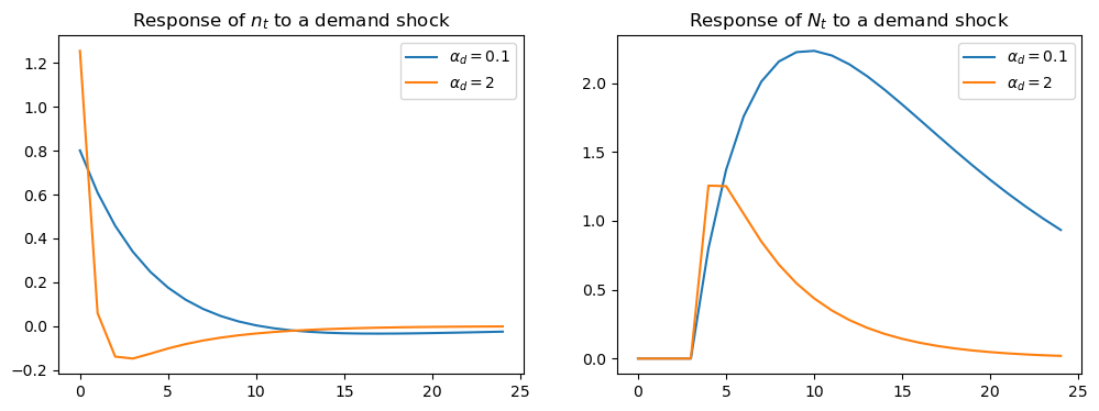
The first figure plots the impulse response of \(n_t\) (on the left) and \(N_t\) (on the right) to a positive demand shock, for \(\alpha_d = 0.1\) and \(\alpha_d = 2\).

When \(\alpha_d = 2\), the number of new students \(n_t\) rises initially, but the response then turns negative.

A positive demand shock raises wages, drawing new students into the profession.

However, these new students raise \(N_t\).

The higher is \(\alpha_d\), the larger the effect of this rise in \(N_t\) on wages.

This counteracts the demand shock’s positive effect on wages, reducing the number of new students in subsequent periods.

Consequently, when \(\alpha_d\) is lower, the effect of a demand shock on \(N_t\) is larger

fig, (ax1, ax2) = plt.subplots(1, 2, figsize=(12, 4))
ax1.plot(econ1.c_irf,label=r'$\alpha_d = 0.1$')
ax1.plot(econ2.c_irf,label=r'$\alpha_d = 2$')
ax1.legend()
ax1.set_title('Response of $n_t$ to a demand shock')

ax2.plot(econ1.h_irf[:, 0], label=r'$\alpha_d = 0.1$')
ax2.plot(econ2.h_irf[:, 0], label=r'$\alpha_d = 2$')
ax2.legend()
ax2.set_title('Response of $N_t$ to a demand shock')
plt.show()

_images/510a2b0ddcb89f725eef4f3a2f60e718ab15b001f1d96010bcd27a82659e7a2c.png

The next figure plots the impulse response of \(n_t\) (on the left) and \(N_t\) (on the right) to a positive demand shock, for \(k=4\), \(k=7\) and \(k=10\) (with \(\alpha_d = 0.1\))

fig, (ax1, ax2) = plt.subplots(1, 2, figsize=(12, 4))
ax1.plot(econ1.c_irf, label='$k=4$')
ax1.plot(econ3.c_irf, label='$k=7$')
ax1.plot(econ4.c_irf, label='$k=10$')
ax1.legend()
ax1.set_title('Response of $n_t$ to a demand shock')

ax2.plot(econ1.h_irf[:,0], label='$k=4$')
ax2.plot(econ3.h_irf[:,0], label='$k=7$')
ax2.plot(econ4.h_irf[:,0], label='$k=10$')
ax2.legend()
ax2.set_title('Response of $N_t$ to a demand shock')
plt.show()

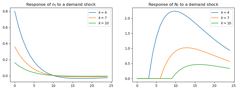
_images/adbaaf3f329f59f6b5ed541e7a09a3fb31802a905cd178fb4ac02f5666264c9a.png

Both panels in the above figure show that raising \(k\) lowers the effect of a positive demand shock on entry into the engineering profession.

Increasing the number of periods of schooling lowers the number of new students in response to a demand shock.

This occurs because with longer required schooling, new students ultimately benefit less from the impact of that shock on wages.

24.3. Exercises#

Exercise 24.1

In the lecture we varied the slope of the demand curve \(\alpha_d\) and the length of schooling \(k\), holding the persistence of the demand shock fixed at \(\rho_d = 0.8\).

Now investigate how the persistence of the demand shock matters.

Holding \(k = 4\) and \(\alpha_d = 0.1\), compute and plot the impulse responses of \(n_t\) and \(N_t\) to a unit demand shock for \(\rho_d \in \{0.2, 0.5, 0.8, 0.95\}\).

You should find that as \(\rho_d\) falls towards zero the responses shrink towards zero, so that a nearly transitory demand shock leaves entry and the engineer stock almost unchanged.

Predict the direction of the effect before running the code, and then explain why a transitory demand shock produces essentially no response.

Solution

Recall that the present value of entering engineering school is

\[ v_t = \beta^k \mathbb{E}_t \sum_{j=0}^\infty (\beta \delta_N)^j w_{t+k+j}. \]

A student who enters at \(t\) does not start earning the wage until \(t+k\).

Ignoring the general-equilibrium feedback through \(N_t\), the wage premium expected \(k+j\) periods ahead is \(\rho_d^{\,k+j}\,\epsilon_{dt}\), so

\[ v_t \;\propto\; (\beta \rho_d)^k\, \epsilon_{dt} \sum_{j=0}^\infty (\beta \delta_N \rho_d)^j . \]

The decisive term is the factor \((\beta \rho_d)^k\) out front: what matters is how much of the wage premium survives the \(k\) periods of schooling.

Hence the more persistent is the demand shock (the larger is \(\rho_d\)), the more of the wage increase remains by graduation, so \(v_t\) — and therefore entry \(n_t\) and ultimately the stock \(N_t\) — responds more strongly.

In the limit \(\rho_d \to 0\) the factor \((\beta\rho_d)^k \to 0\): a purely transitory demand shock has fully died out (in expectation) before any new student can graduate, so \(v_t = 0\) and there is no response of \(n_t\) or \(N_t\) at all. This is the sharpest expression of the time-to-build mechanism.

We rebuild the model for \(k = 4\) and loop over values of \(\rho_d\).

k = 4

β = np.array([[1 / 1.05]])
α_d = np.array([[0.1]])
α_s = 1
ε_1 = 1e-7
λ_1 = np.full((1, k), ε_1)
l_λ = np.hstack((α_d, λ_1))
π_h = np.array([[0]])

δ_n = np.array([[0.95]])
d1 = np.vstack((δ_n, np.zeros((k - 1, 1))))
d2 = np.hstack((d1, np.eye(k)))
δ_h = np.vstack((d2, np.zeros((1, k + 1))))
θ_h = np.vstack((np.zeros((k, 1)), np.ones((1, 1))))

ψ_1 = 1 / α_s
ϕ_c = np.array([[1], [0]])
ϕ_g = np.array([[0], [-1]])
ϕ_i = np.array([[-1], [ψ_1]])
γ = np.array([[0], [0]])
δ_k = np.array([[0]])
θ_k = np.array([[0]])

ρ_s = 0.8
c2 = np.array([[0, 0], [10, 0], [0, 10]])
ub = np.array([[30, 0, 1]])
ud = np.array([[10, 1, 0], [0, 0, 0]])

pref = Preferences(β, l_λ, π_h, δ_h, θ_h)
tech = Technology(ϕ_c, ϕ_g, ϕ_i, γ, δ_k, θ_k)

shock_demand = np.array([[0], [1]])

fig, (ax1, ax2) = plt.subplots(1, 2, figsize=(12, 4))

for ρ_d in [0.2, 0.5, 0.8, 0.95]:
    a22 = np.array([[1,   0,   0],
                    [0, ρ_s,   0],
                    [0,   0, ρ_d]])
    info = Information(a22, c2, ub, ud)
    econ = DLE(info, tech, pref)
    econ.irf(ts_length=25, shock=shock_demand)
    ax1.plot(econ.c_irf, label=fr'$\rho_d = {ρ_d}$')
    ax2.plot(econ.h_irf[:, 0], label=fr'$\rho_d = {ρ_d}$')

ax1.legend()
ax1.set_title('Response of $n_t$ to a demand shock')
ax2.legend()
ax2.set_title('Response of $N_t$ to a demand shock')
plt.show()

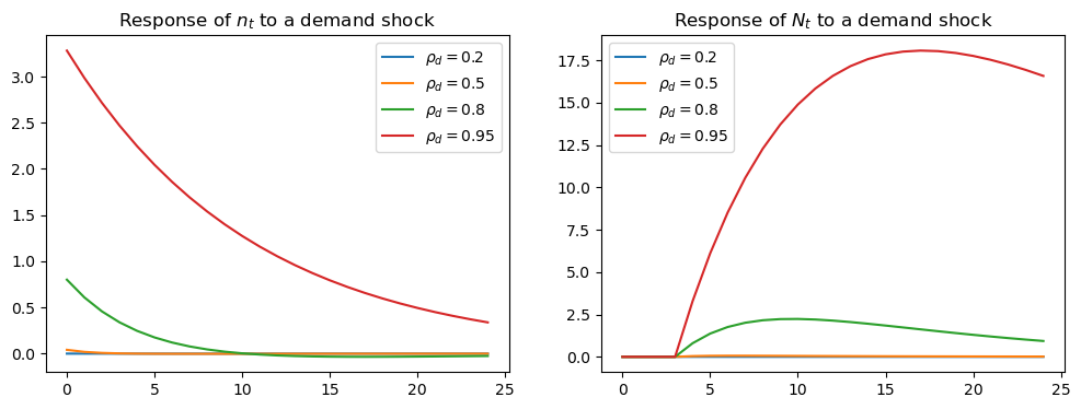
_images/670c89c93f968ed920373391196db2ae6009440515968ae41871401e0ee9f295.png

As anticipated, a more persistent demand shock produces a larger response of both entry \(n_t\) and the stock of engineers \(N_t\).

Notice how steeply the responses fall as \(\rho_d\) declines: the \(\rho_d = 0.2\) curves sit almost on top of the zero line. This is the \((\beta\rho_d)^k\) factor at work — with \(k = 4\) and \(\beta \approx 0.95\) we have \((\beta \times 0.2)^4 \approx 0.0013\) against \((\beta \times 0.95)^4 \approx 0.67\), so the \(\rho_d = 0.2\) response is only about two tenths of one percent of the \(\rho_d = 0.95\) response.

When \(\rho_d\) is small the wage increase has largely dissipated by the time a new student graduates \(k\) periods later, so the incentive to enter is weak — and for a purely transitory shock (\(\rho_d = 0\)) it disappears entirely.

Exercise 24.2

The slope of Ryoo and Rosen’s supply curve is governed by \(\alpha_s\), which enters the household technology through \(\psi_1 = 1 / \alpha_s\).

Holding \(k = 4\), \(\alpha_d = 0.1\) and \(\rho_d = 0.8\), compute and plot the impulse responses of \(n_t\) and \(N_t\) to a unit demand shock for \(\alpha_s \in \{0.5, 1, 2\}\).

Explain the economic intuition for what you find.

Solution

A larger \(\alpha_s\) means a flatter (more elastic) supply curve of new students, so a given rise in the present value \(v_t\) of entering the profession draws in more new students.

We therefore expect the response of \(n_t\) — and, with a lag, the response of \(N_t\) — to grow as \(\alpha_s\) increases.

k = 4

β = np.array([[1 / 1.05]])
α_d = np.array([[0.1]])
ε_1 = 1e-7
λ_1 = np.full((1, k), ε_1)
l_λ = np.hstack((α_d, λ_1))
π_h = np.array([[0]])

δ_n = np.array([[0.95]])
d1 = np.vstack((δ_n, np.zeros((k - 1, 1))))
d2 = np.hstack((d1, np.eye(k)))
δ_h = np.vstack((d2, np.zeros((1, k + 1))))
θ_h = np.vstack((np.zeros((k, 1)), np.ones((1, 1))))

γ = np.array([[0], [0]])
δ_k = np.array([[0]])
θ_k = np.array([[0]])

ρ_s = 0.8
ρ_d = 0.8
a22 = np.array([[1,   0,   0],
                [0, ρ_s,   0],
                [0,   0, ρ_d]])
c2 = np.array([[0, 0], [10, 0], [0, 10]])
ub = np.array([[30, 0, 1]])
ud = np.array([[10, 1, 0], [0, 0, 0]])

info = Information(a22, c2, ub, ud)
pref = Preferences(β, l_λ, π_h, δ_h, θ_h)

shock_demand = np.array([[0], [1]])

fig, (ax1, ax2) = plt.subplots(1, 2, figsize=(12, 4))

for α_s in [0.5, 1, 2]:
    ψ_1 = 1 / α_s
    ϕ_c = np.array([[1], [0]])
    ϕ_g = np.array([[0], [-1]])
    ϕ_i = np.array([[-1], [ψ_1]])
    tech = Technology(ϕ_c, ϕ_g, ϕ_i, γ, δ_k, θ_k)
    econ = DLE(info, tech, pref)
    econ.irf(ts_length=25, shock=shock_demand)
    ax1.plot(econ.c_irf, label=fr'$\alpha_s = {α_s}$')
    ax2.plot(econ.h_irf[:, 0], label=fr'$\alpha_s = {α_s}$')

ax1.legend()
ax1.set_title('Response of $n_t$ to a demand shock')
ax2.legend()
ax2.set_title('Response of $N_t$ to a demand shock')
plt.show()

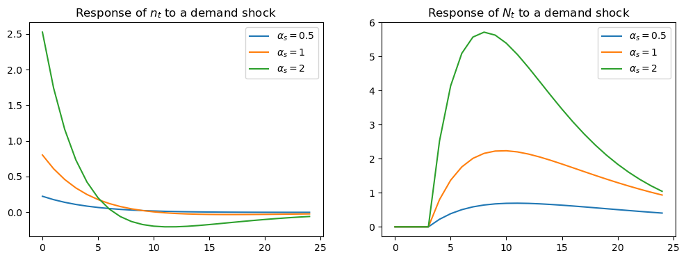
_images/345b2128b5ca8e84eaa84eab9876326712e5eb8f004fc9b41d426cd18761b55b.png

The figures confirm the intuition: a more elastic supply of students (a larger \(\alpha_s\)) amplifies the response of new entrants \(n_t\) to the demand shock, and this feeds through into a larger response of the stock of engineers \(N_t\).