44. Two Modifications of Mean-Variance Portfolio Theory#
44.1. Overview#
This lecture describes extensions to the classical mean-variance portfolio theory summarized in our lecture Elementary Asset Pricing Theory.
The classic theory described there assumes that a decision maker completely trusts the statistical model that he posits to govern the joint distribution of returns on a list of available assets.
Both extensions described here put distrust of that statistical model into the mind of the decision maker.
One is a model of Black and Litterman [Black and Litterman, 1992] that imputes to the decision maker distrust of historically estimated mean returns but still complete trust of estimated covariances of returns.
The second model also imputes to the decision maker doubts about his statistical model, but now by saying that, because of that distrust, the decision maker uses a version of robust control theory described in this lecture Robustness.
The famous Black-Litterman (1992) [Black and Litterman, 1992] portfolio choice model was motivated by the finding that with high frequency or moderately high frequency data, means are more difficult to estimate than variances.
A model of robust portfolio choice that we’ll describe below also begins from the same starting point.
To begin, we’ll take for granted that means are more difficult to estimate that covariances and will focus on how Black and Litterman, on the one hand, an robust control theorists, on the other, would recommend modifying the mean-variance portfolio choice model to take that into account.
At the end of this lecture, we shall use some rates of convergence results and some simulations to verify how means are more difficult to estimate than variances.
Among the ideas in play in this lecture will be
Mean-variance portfolio theory
Bayesian approaches to estimating linear regressions
A risk-sensitivity operator and its connection to robust control theory
In summary, we’ll describe two ways to modify the classic mean-variance portfolio choice model in ways designed to make its recommendations more plausible.
Both of the adjustments that we describe are designed to confront a widely recognized embarrassment to mean-variance portfolio theory, namely, that it usually implies taking very extreme long-short portfolio positions.
The two approaches build on a common and widespread hunch – that because it is much easier statistically to estimate covariances of excess returns than it is to estimate their means, it makes sense to adjust investors’ subjective beliefs about mean returns in order to render more plausible decisions.
Let’s start with some imports:
import numpy as np
import scipy.stats as stat
import matplotlib.pyplot as plt
from numba import jit
44.2. Mean-variance portfolio choice#
A risk-free security earns one-period net return \(r_f\).
An \(n \times 1\) vector of risky securities earns an \(n \times 1\) vector \(\vec r - r_f {\bf 1}\) of excess returns, where \({\bf 1}\) is an \(n \times 1\) vector of ones.
The excess return vector is multivariate normal with mean \(\mu\) and covariance matrix \(\Sigma\), which we express either as
or
where \(\epsilon \sim {\mathcal N}(0, I)\) is an \(n \times 1\) random vector.
Let \(w\) be an \(n \times 1\) vector of portfolio weights.
A portfolio consisting \(w\) earns returns
The mean-variance portfolio choice problem is to choose \(w\) to maximize
where \(\delta > 0\) is a risk-aversion parameter. The first-order condition for maximizing (44.1) with respect to the vector \(w\) is
which implies the following design of a risky portfolio:
44.3. Estimating mean and variance#
The key inputs into the portfolio choice model (44.2) are
estimates of the parameters \(\mu, \Sigma\) of the random excess return vector\((\vec r - r_f {\bf 1})\)
the risk-aversion parameter \(\delta\)
A standard way of estimating \(\mu\) is maximum-likelihood or least squares; that amounts to estimating \(\mu\) by a sample mean of excess returns and estimating \(\Sigma\) by a sample covariance matrix.
44.4. Black-Litterman starting point#
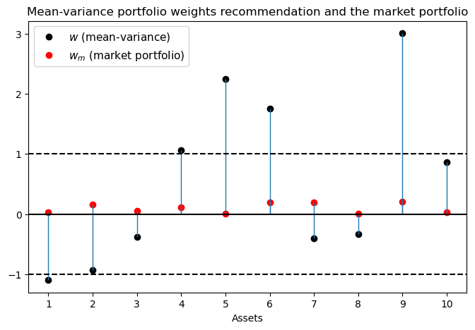
When estimates of \(\mu\) and \(\Sigma\) from historical sample means and covariances have been combined with plausible values of the risk-aversion parameter \(\delta\) to compute an optimal portfolio from formula (44.2), a typical outcome has been \(w\)’s with extreme long and short positions.
A common reaction to these outcomes is that they are so implausible that a portfolio manager cannot recommend them to a customer.
np.random.seed(12)

N = 10                                           # Number of assets
T = 200                                          # Sample size

# random market portfolio (sum is normalized to 1)
w_m = np.random.rand(N)
w_m = w_m / (w_m.sum())

# True risk premia and variance of excess return (constructed
# so that the Sharpe ratio is 1)
μ = (np.random.randn(N) + 5)  /100      # Mean excess return (risk premium)
S = np.random.randn(N, N)        # Random matrix for the covariance matrix
V = S @ S.T           # Turn the random matrix into symmetric psd
# Make sure that the Sharpe ratio is one
Σ = V * (w_m @ μ)**2 / (w_m @ V @ w_m)

# Risk aversion of market portfolio holder
δ = 1 / np.sqrt(w_m @ Σ @ w_m)

# Generate a sample of excess returns
excess_return = stat.multivariate_normal(μ, Σ)
sample = excess_return.rvs(T)

# Estimate μ and Σ
μ_est = sample.mean(0).reshape(N, 1)
Σ_est = np.cov(sample.T)

w = np.linalg.solve(δ * Σ_est, μ_est)

fig, ax = plt.subplots(figsize=(8, 5))
ax.set_title('Mean-variance portfolio weights recommendation and the market portfolio')
ax.plot(np.arange(N)+1, w, 'o', c='k', label='$w$ (mean-variance)')
ax.plot(np.arange(N)+1, w_m, 'o', c='r', label='$w_m$ (market portfolio)')
ax.vlines(np.arange(N)+1, 0, w, lw=1)
ax.vlines(np.arange(N)+1, 0, w_m, lw=1)
ax.axhline(0, c='k')
ax.axhline(-1, c='k', ls='--')
ax.axhline(1, c='k', ls='--')
ax.set_xlabel('Assets')
ax.xaxis.set_ticks(np.arange(1, N+1, 1))
plt.legend(numpoints=1, fontsize=11)
plt.show()
Black and Litterman’s responded to this situation in the following way:
They continue to accept (44.2) as a good model for choosing an optimal portfolio \(w\).
They want to continue to allow the customer to express his or her risk tolerance by setting \(\delta\).
Leaving \(\Sigma\) at its maximum-likelihood value, they push \(\mu\) away from its maximum-likelihood value in a way designed to make portfolio choices that are more plausible in terms of conforming to what most people actually do.
In particular, given \(\Sigma\) and a plausible value of \(\delta\), Black and Litterman reverse engineered a vector \(\mu_{BL}\) of mean excess returns that makes the \(w\) implied by formula (44.2) equal the actual market portfolio \(w_m\), so that
44.5. Details#
Let’s define
as the (scalar) excess return on the market portfolio \(w_m\).
Define
as the variance of the excess return on the market portfolio \(w_m\).
Define
as the Sharpe-ratio on the market portfolio \(w_m\).
Let \(\delta_m\) be the value of the risk aversion parameter that induces an investor to hold the market portfolio in light of the optimal portfolio choice rule (44.2).
Evidently, portfolio rule (44.2) then implies that \(r_m - r_f = \delta_m \sigma^2\) or
or
Following the Black-Litterman philosophy, our first step will be to back a value of \(\delta_m\) from
an estimate of the Sharpe-ratio, and
our maximum likelihood estimate of \(\sigma\) drawn from our estimates or \(w_m\) and \(\Sigma\)
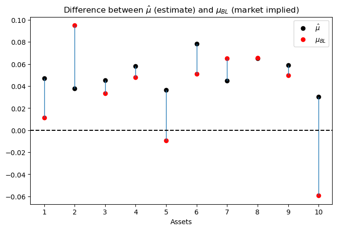
The second key Black-Litterman step is then to use this value of \(\delta\) together with the maximum likelihood estimate of \(\Sigma\) to deduce a \(\mu_{\bf BL}\) that verifies portfolio rule (44.2) at the market portfolio \(w = w_m\)
The starting point of the Black-Litterman portfolio choice model is thus a pair \((\delta_m, \mu_m)\) that tells the customer to hold the market portfolio.
# Observed mean excess market return
r_m = w_m @ μ_est

# Estimated variance of the market portfolio
σ_m = w_m @ Σ_est @ w_m

# Sharpe-ratio
sr_m = r_m / np.sqrt(σ_m)

# Risk aversion of market portfolio holder
d_m = r_m / σ_m

# Derive "view" which would induce the market portfolio
μ_m = (d_m * Σ_est @ w_m).reshape(N, 1)

x = np.arange(N) + 1
fig, ax = plt.subplots(figsize=(8, 5))
ax.set_title(r'Difference between $\hat{\mu}$ (estimate) and $\mu_{BL}$ (market implied)')
ax.plot(x, μ_est, 'o', c='k', label=r'$\hat{\mu}$')
ax.plot(x, μ_m, 'o', c='r', label=r'$\mu_{BL}$')
ax.vlines(x, μ_m, μ_est, lw=1)
ax.axhline(0, c='k', ls='--')
ax.set_xlabel('Assets')
ax.xaxis.set_ticks(np.arange(1, N+1, 1))
plt.legend(numpoints=1)
plt.show()
44.6. Adding views#
Black and Litterman start with a baseline customer who asserts that he or she shares the market’s views, which means that he or she believes that excess returns are governed by
Black and Litterman would advise that customer to hold the market portfolio of risky securities.
Black and Litterman then imagine a consumer who would like to express a view that differs from the market’s.
The consumer wants appropriately to mix his view with the market’s before using (44.2) to choose a portfolio.
Suppose that the customer’s view is expressed by a hunch that rather than (44.3), excess returns are governed by
where \(\tau > 0\) is a scalar parameter that determines how the decision maker wants to mix his view \(\hat \mu\) with the market’s view \(\mu_{\bf BL}\).
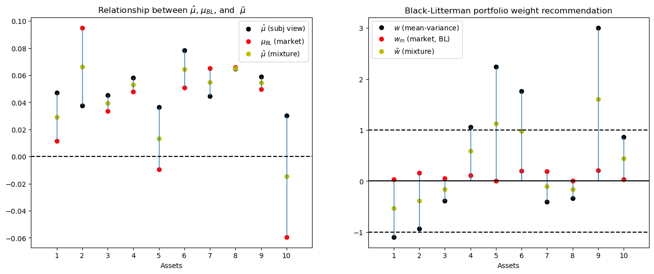
Black and Litterman would then use a formula like the following one to mix the views \(\hat \mu\) and \(\mu_{\bf BL}\)
Black and Litterman would then advise the customer to hold the portfolio associated with these views implied by rule (44.2):
This portfolio \(\tilde w\) will deviate from the portfolio \(w_{BL}\) in amounts that depend on the mixing parameter \(\tau\).
If \(\hat \mu\) is the maximum likelihood estimator and \(\tau\) is chosen heavily to weight this view, then the customer’s portfolio will involve big short-long positions.
def black_litterman(λ, μ1, μ2, Σ1, Σ2):
    """
    This function calculates the Black-Litterman mixture
    mean excess return and covariance matrix
    """
    Σ1_inv = np.linalg.inv(Σ1)
    Σ2_inv = np.linalg.inv(Σ2)

    μ_tilde = np.linalg.solve(Σ1_inv + λ * Σ2_inv,
                              Σ1_inv @ μ1 + λ * Σ2_inv @ μ2)
    return μ_tilde

τ = 1
μ_tilde = black_litterman(1, μ_m, μ_est, Σ_est, τ * Σ_est)

# The Black-Litterman recommendation for the portfolio weights
w_tilde = np.linalg.solve(δ * Σ_est, μ_tilde)
def BL_plot(τ):
    μ_tilde = black_litterman(1, μ_m, μ_est, Σ_est, τ * Σ_est)
    w_tilde = np.linalg.solve(δ * Σ_est, μ_tilde)

    fig, ax = plt.subplots(1, 2, figsize=(16, 6))
    ax[0].plot(np.arange(N)+1, μ_est, 'o', c='k',
               label=r'$\hat{\mu}$ (subj view)')
    ax[0].plot(np.arange(N)+1, μ_m, 'o', c='r',
               label=r'$\mu_{BL}$ (market)')
    ax[0].plot(np.arange(N)+1, μ_tilde, 'o', c='y',
               label=r'$\tilde{\mu}$ (mixture)')
    ax[0].vlines(np.arange(N)+1, μ_m, μ_est, lw=1)
    ax[0].axhline(0, c='k', ls='--')
    ax[0].set(xlim=(0, N+1), xlabel='Assets',
              title=r'Relationship between $\hat{\mu}$, $\mu_{BL}$, and  $ \tilde{\mu}$')
    ax[0].xaxis.set_ticks(np.arange(1, N+1, 1))
    ax[0].legend(numpoints=1)

    ax[1].set_title('Black-Litterman portfolio weight recommendation')
    ax[1].plot(np.arange(N)+1, w, 'o', c='k', label=r'$w$ (mean-variance)')
    ax[1].plot(np.arange(N)+1, w_m, 'o', c='r', label=r'$w_{m}$ (market, BL)')
    ax[1].plot(np.arange(N)+1, w_tilde, 'o', c='y',
               label=r'$\tilde{w}$ (mixture)')
    ax[1].vlines(np.arange(N)+1, 0, w, lw=1)
    ax[1].vlines(np.arange(N)+1, 0, w_m, lw=1)
    ax[1].axhline(0, c='k')
    ax[1].axhline(-1, c='k', ls='--')
    ax[1].axhline(1, c='k', ls='--')
    ax[1].set(xlim=(0, N+1), xlabel='Assets',
              title='Black-Litterman portfolio weight recommendation')
    ax[1].xaxis.set_ticks(np.arange(1, N+1, 1))
    ax[1].legend(numpoints=1)
    plt.show()

BL_plot(τ)
44.7. Bayesian interpretation#
Consider the following Bayesian interpretation of the Black-Litterman recommendation.
The prior belief over the mean excess returns is consistent with the market portfolio and is given by
Given a particular realization of the mean excess returns \(\mu\) one observes the average excess returns \(\hat \mu\) on the market according to the distribution
where \(\tau\) is typically small capturing the idea that the variation in the mean is smaller than the variation of the individual random variable.
Given the realized excess returns one should then update the prior over the mean excess returns according to Bayes rule.
The corresponding posterior over mean excess returns is normally distributed with mean
The covariance matrix is
Hence, the Black-Litterman recommendation is consistent with the Bayes update of the prior over the mean excess returns in light of the realized average excess returns on the market.
44.8. Curve decolletage#
Consider two independent “competing” views on the excess market returns
and
A special feature of the multivariate normal random variable \(Z\) is that its density function depends only on the (Euclidiean) length of its realization \(z\).
Formally, let the \(k\)-dimensional random vector be
then
and so the points where the density takes the same value can be described by the ellipse
where \(\bar d\in\mathbb{R}_+\) denotes the (transformation) of a particular density value.
The curves defined by equation (44.5) can be labeled as iso-likelihood ellipses
Remark: More generally there is a class of density functions that possesses this feature, i.e.
\[ \exists g: \mathbb{R}_+ \mapsto \mathbb{R}_+ \ \ \text{ and } \ \ c \geq 0, \ \ \text{s.t. the density } \ \ f \ \ \text{of} \ \ Z \ \ \text{ has the form } \quad f(z) = c g(z\cdot z) \]This property is called spherical symmetry (see p 81. in Leamer (1978) [Leamer, 1978]).
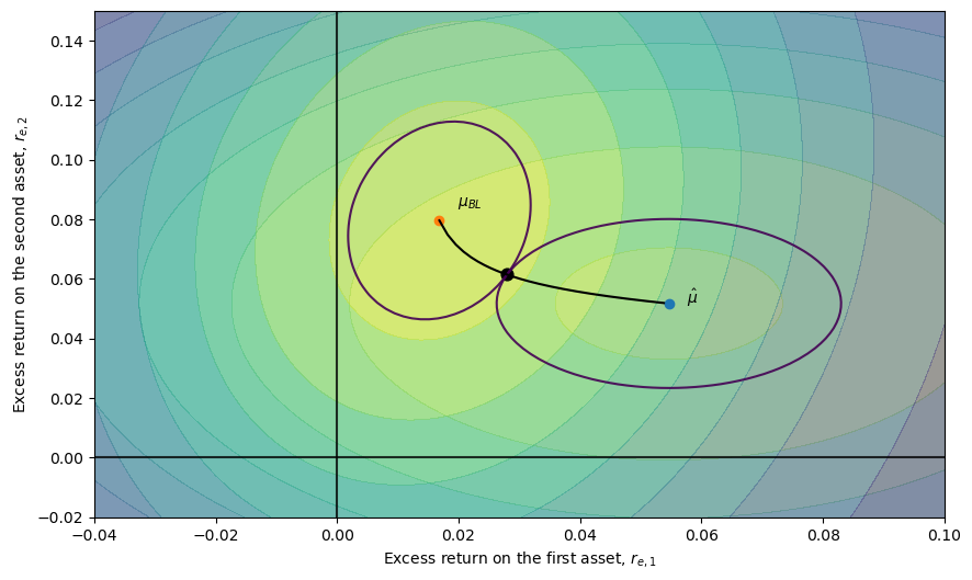
In our specific example, we can use the pair \((\bar d_1, \bar d_2)\) as being two “likelihood” values for which the corresponding iso-likelihood ellipses in the excess return space are given by
Notice that for particular \(\bar d_1\) and \(\bar d_2\) values the two ellipses have a tangency point.
These tangency points, indexed by the pairs \((\bar d_1, \bar d_2)\), characterize points \(\vec r_e\) from which there exists no deviation where one can increase the likelihood of one view without decreasing the likelihood of the other view.
The pairs \((\bar d_1, \bar d_2)\) for which there is such a point outlines a curve in the excess return space. This curve is reminiscent of the Pareto curve in an Edgeworth-box setting.
Dickey (1975) [Dickey, 1975] calls it a curve decolletage.
Leamer (1978) [Leamer, 1978] calls it an information contract curve and describes it by the following program: maximize the likelihood of one view, say the Black-Litterman recommendation while keeping the likelihood of the other view at least at a prespecified constant \(\bar d_2\)
Denoting the multiplier on the constraint by \(\lambda\), the first-order condition is
which defines the information contract curve between \(\mu_{BL}\) and \(\hat \mu\)
Note that if \(\lambda = 1\), (44.6) is equivalent with (44.4) and it identifies one point on the information contract curve.
Furthermore, because \(\lambda\) is a function of the minimum likelihood \(\bar d_2\) on the RHS of the constraint, by varying \(\bar d_2\) (or \(\lambda\) ), we can trace out the whole curve as the figure below illustrates.
np.random.seed(1987102)

N = 2                                           # Number of assets
T = 200                                         # Sample size
τ = 0.8

# Random market portfolio (sum is normalized to 1)
w_m = np.random.rand(N)
w_m = w_m / (w_m.sum())

μ = (np.random.randn(N) + 5) / 100
S = np.random.randn(N, N)
V = S @ S.T
Σ = V * (w_m @ μ)**2 / (w_m @ V @ w_m)

excess_return = stat.multivariate_normal(μ, Σ)
sample = excess_return.rvs(T)

μ_est = sample.mean(0).reshape(N, 1)
Σ_est = np.cov(sample.T)

σ_m = w_m @ Σ_est @ w_m
d_m = (w_m @ μ_est) / σ_m
μ_m = (d_m * Σ_est @ w_m).reshape(N, 1)

N_r1, N_r2 = 100, 100
r1 = np.linspace(-0.04, .1, N_r1)
r2 = np.linspace(-0.02, .15, N_r2)

λ_grid = np.linspace(.001, 20, 100)
curve = np.asarray([black_litterman(λ, μ_m, μ_est, Σ_est,
                                    τ * Σ_est).flatten() for λ in λ_grid])

λ = 1
def decolletage(λ):
    dist_r_BL = stat.multivariate_normal(μ_m.squeeze(), Σ_est)
    dist_r_hat = stat.multivariate_normal(μ_est.squeeze(), τ * Σ_est)

    X, Y = np.meshgrid(r1, r2)
    XY = np.stack((X, Y), axis=-1)
    Z_BL = dist_r_BL.pdf(XY)
    Z_hat = dist_r_hat.pdf(XY)

    μ_tilde = black_litterman(λ, μ_m, μ_est, Σ_est, τ * Σ_est).flatten()

    fig, ax = plt.subplots(figsize=(10, 6))
    ax.contourf(X, Y, Z_hat, cmap='viridis', alpha =.4)
    ax.contourf(X, Y, Z_BL, cmap='viridis', alpha =.4)
    ax.contour(X, Y, Z_BL, [dist_r_BL.pdf(μ_tilde)], cmap='viridis', alpha=.9)
    ax.contour(X, Y, Z_hat, [dist_r_hat.pdf(μ_tilde)], cmap='viridis', alpha=.9)
    ax.scatter(μ_est[0], μ_est[1])
    ax.scatter(μ_m[0], μ_m[1])
    ax.scatter(μ_tilde[0], μ_tilde[1], c='k', s=20*3)

    ax.plot(curve[:, 0], curve[:, 1], c='k')
    ax.axhline(0, c='k', alpha=.8)
    ax.axvline(0, c='k', alpha=.8)
    ax.set_xlabel(r'Excess return on the first asset, $r_{e, 1}$')
    ax.set_ylabel(r'Excess return on the second asset, $r_{e, 2}$')
    ax.text(μ_est[0] + 0.003, μ_est[1], r'$\hat{\mu}$')
    ax.text(μ_m[0] + 0.003, μ_m[1] + 0.005, r'$\mu_{BL}$')
    plt.show()

decolletage(λ)
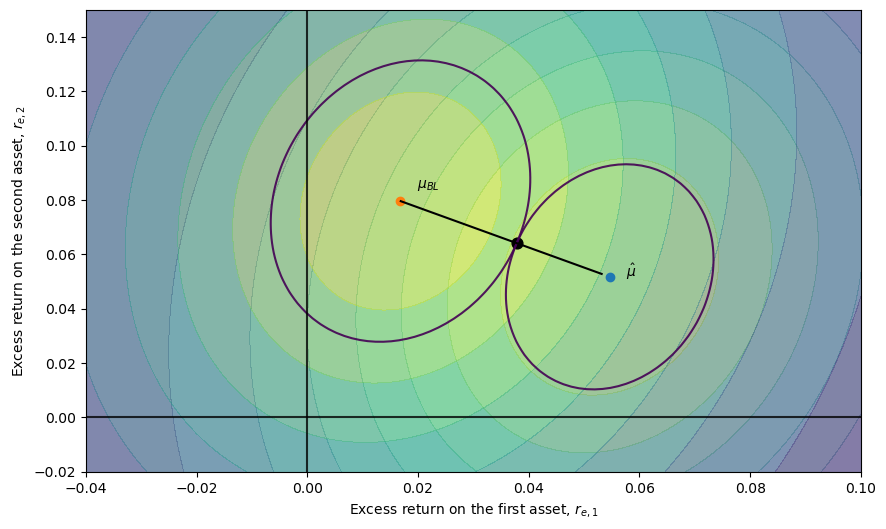
Note that the line that connects the two points \(\hat \mu\) and \(\mu_{BL}\) is linear, which comes from the fact that the covariance matrices of the two competing distributions (views) are proportional to each other.
To illustrate the fact that this is not necessarily the case, consider another example using the same parameter values, except that the “second view” constituting the constraint has covariance matrix \(\tau I\) instead of \(\tau \Sigma\).
This leads to the following figure, on which the curve connecting \(\hat \mu\) and \(\mu_{BL}\) are bending
λ_grid = np.linspace(.001, 20000, 1000)
curve = np.asarray([black_litterman(λ, μ_m, μ_est, Σ_est,
                                    τ * np.eye(N)).flatten() for λ in λ_grid])
λ = 200
def decolletage(λ):
    dist_r_BL = stat.multivariate_normal(μ_m.squeeze(), Σ_est)
    dist_r_hat = stat.multivariate_normal(μ_est.squeeze(), τ * np.eye(N))

    X, Y = np.meshgrid(r1, r2)
    XY = np.stack((X, Y), axis=-1)
    Z_BL = dist_r_BL.pdf(XY)
    Z_hat = dist_r_hat.pdf(XY)

    μ_tilde = black_litterman(λ, μ_m, μ_est, Σ_est, τ * np.eye(N)).flatten()

    fig, ax = plt.subplots(figsize=(10, 6))
    ax.contourf(X, Y, Z_hat, cmap='viridis', alpha=.4)
    ax.contourf(X, Y, Z_BL, cmap='viridis', alpha=.4)
    ax.contour(X, Y, Z_BL, [dist_r_BL.pdf(μ_tilde)], cmap='viridis', alpha=.9)
    ax.contour(X, Y, Z_hat, [dist_r_hat.pdf(μ_tilde)], cmap='viridis', alpha=.9)
    ax.scatter(μ_est[0], μ_est[1])
    ax.scatter(μ_m[0], μ_m[1])

    ax.scatter(μ_tilde[0], μ_tilde[1], c='k', s=20*3)

    ax.plot(curve[:, 0], curve[:, 1], c='k')
    ax.axhline(0, c='k', alpha=.8)
    ax.axvline(0, c='k', alpha=.8)
    ax.set_xlabel(r'Excess return on the first asset, $r_{e, 1}$')
    ax.set_ylabel(r'Excess return on the second asset, $r_{e, 2}$')
    ax.text(μ_est[0] + 0.003, μ_est[1], r'$\hat{\mu}$')
    ax.text(μ_m[0] + 0.003, μ_m[1] + 0.005, r'$\mu_{BL}$')
    plt.show()

decolletage(λ)
44.9. Black-Litterman recommendation as regularization#
First, consider the OLS regression
which yields the solution
A common performance measure of estimators is the mean squared error (MSE).
An estimator is “good” if its MSE is relatively small. Suppose that \(\beta_0\) is the “true” value of the coefficient, then the MSE of the OLS estimator is
From this decomposition, one can see that in order for the MSE to be small, both the bias and the variance terms must be small.
For example, consider the case when \(X\) is a \(T\)-vector of ones (where \(T\) is the sample size), so \(\hat\beta_{OLS}\) is simply the sample average, while \(\beta_0\in \mathbb{R}\) is defined by the true mean of \(y\).
In this example the MSE is
However, because there is a trade-off between the estimator’s bias and variance, there are cases when by permitting a small bias we can substantially reduce the variance so overall the MSE gets smaller.
A typical scenario when this proves to be useful is when the number of coefficients to be estimated is large relative to the sample size.
In these cases, one approach to handle the bias-variance trade-off is the so called Tikhonov regularization.
A general form with regularization matrix \(\Gamma\) can be written as
which yields the solution
Substituting the value of \(\hat{\beta}_{OLS}\) yields
Often, the regularization matrix takes the form \(\Gamma = \lambda I\) with \(\lambda>0\) and \(\tilde \beta = \mathbf{0}\).
Then the Tikhonov regularization is equivalent to what is called ridge regression in statistics.
To illustrate how this estimator addresses the bias-variance trade-off, we compute the MSE of the ridge estimator
The ridge regression shrinks the coefficients of the estimated vector towards zero relative to the OLS estimates thus reducing the variance term at the cost of introducing a “small” bias.
However, there is nothing special about the zero vector.
When \(\tilde \beta \neq \mathbf{0}\) shrinkage occurs in the direction of \(\tilde \beta\).
Now, we can give a regularization interpretation of the Black-Litterman portfolio recommendation.
To this end, first simplify the equation (44.4) that characterizes the Black-Litterman recommendation
In our case, \(\hat \mu\) is the estimated mean excess returns of securities. This could be written as a vector autoregression where
\(y\) is the stacked vector of observed excess returns of size \((N T\times 1)\) – \(N\) securities and \(T\) observations.
\(X = \sqrt{T^{-1}}(I_{N} \otimes \iota_T)\) where \(I_N\) is the identity matrix and \(\iota_T\) is a column vector of ones.
Correspondingly, the OLS regression of \(y\) on \(X\) would yield the mean excess returns as coefficients.
With \(\Gamma = \sqrt{\tau T^{-1}}(I_{N} \otimes \iota_T)\) we can write the regularized version of the mean excess return estimation
Given that \(\hat \beta_{OLS} = \hat \mu\) and \(\tilde \beta = \mu_{BL}\) in the Black-Litterman model, we have the following interpretation of the model’s recommendation.
The estimated (personal) view of the mean excess returns, \(\hat{\mu}\) that would lead to extreme short-long positions are “shrunk” towards the conservative market view, \(\mu_{BL}\), that leads to the more conservative market portfolio.
So the Black-Litterman procedure results in a recommendation that is a compromise between the conservative market portfolio and the more extreme portfolio that is implied by estimated “personal” views.
44.10. A robust control operator#
The Black-Litterman approach is partly inspired by the econometric insight that it is easier to estimate covariances of excess returns than the means.
That is what gave Black and Litterman license to adjust investors’ perception of mean excess returns while not tampering with the covariance matrix of excess returns.
The robust control theory is another approach that also hinges on adjusting mean excess returns but not covariances.
Associated with a robust control problem is what Hansen and Sargent [Hansen and Sargent, 2001], [Hansen and Sargent, 2008] call a \({\sf T}\) operator.
Let’s define the \({\sf T}\) operator as it applies to the problem at hand.
Let \(x\) be an \(n \times 1\) Gaussian random vector with mean vector \(\mu\) and covariance matrix \(\Sigma = C C'\). This means that \(x\) can be represented as
where \(\epsilon \sim {\mathcal N}(0,I)\).
Let \(\phi(\epsilon)\) denote the associated standardized Gaussian density.
Let \(m(\epsilon,\mu)\) be a likelihood ratio, meaning that it satisfies
\(m(\epsilon, \mu) > 0\)
\(\int m(\epsilon,\mu) \phi(\epsilon) d \epsilon =1\)
That is, \(m(\epsilon, \mu)\) is a non-negative random variable with mean 1.
Multiplying \(\phi(\epsilon)\) by the likelihood ratio \(m(\epsilon, \mu)\) produces a distorted distribution for \(\epsilon\), namely
The next concept that we need is the entropy of the distorted distribution \(\tilde \phi\) with respect to \(\phi\).
Entropy is defined as
or
That is, relative entropy is the expected value of the likelihood ratio \(m\) where the expectation is taken with respect to the twisted density \(\tilde \phi\).
Relative entropy is non-negative. It is a measure of the discrepancy between two probability distributions.
As such, it plays an important role in governing the behavior of statistical tests designed to discriminate one probability distribution from another.
We are ready to define the \({\sf T}\) operator.
Let \(V(x)\) be a value function.
Define
This asserts that \({\sf T}\) is an indirect utility function for a minimization problem in which an adversary chooses a distorted probability distribution \(\tilde \phi\) to lower expected utility, subject to a penalty term that gets bigger the larger is relative entropy.
Here the penalty parameter
is a robustness parameter when it is \(+\infty\), there is no scope for the minimizing agent to distort the distribution, so no robustness to alternative distributions is acquired.
As \(\theta\) is lowered, more robustness is achieved.
Note
The \({\sf T}\) operator is sometimes called a risk-sensitivity operator.
We shall apply \({\sf T}\) to the special case of a linear value function \(w'(\vec r - r_f 1)\) where \(\vec r - r_f 1 \sim {\mathcal N}(\mu,\Sigma)\) or \(\vec r - r_f {\bf 1} = \mu + C \epsilon\) and \(\epsilon \sim {\mathcal N}(0,I)\).
The associated worst-case distribution of \(\epsilon\) is Gaussian with mean \(v =-\theta^{-1} C' w\) and covariance matrix \(I\)
(When the value function is affine, the worst-case distribution distorts the mean vector of \(\epsilon\) but not the covariance matrix of \(\epsilon\)).
For utility function argument \(w'(\vec r - r_f 1)\)
and entropy is
44.11. A robust mean-variance portfolio model#
According to criterion (44.1), the mean-variance portfolio choice problem chooses \(w\) to maximize
which equals
A robust decision maker can be modeled as replacing the mean return \(E [w ( \vec r - r_f {\bf 1})]\) with the risk-sensitive criterion
that comes from replacing the mean \(\mu\) of \(\vec r - r\_f {\bf 1}\) with the worst-case mean
Notice how the worst-case mean vector depends on the portfolio \(w\).
The operator \({\sf T}\) is the indirect utility function that emerges from solving a problem in which an agent who chooses probabilities does so in order to minimize the expected utility of a maximizing agent (in our case, the maximizing agent chooses portfolio weights \(w\)).
The robust version of the mean-variance portfolio choice problem is then to choose a portfolio \(w\) that maximizes
or
The minimizer of (44.7) is
where \(\gamma \equiv \theta^{-1}\) is sometimes called the risk-sensitivity parameter.
An increase in the risk-sensitivity parameter \(\gamma\) shrinks the portfolio weights toward zero in the same way that an increase in risk aversion does.
44.12. Appendix#
We want to illustrate the “folk theorem” that with high or moderate frequency data, it is more difficult to estimate means than variances.
In order to operationalize this statement, we take two analog estimators:
sample average: \(\bar X_N = \frac{1}{N}\sum_{i=1}^{N} X_i\)
sample variance: \(S_N = \frac{1}{N-1}\sum_{t=1}^{N} (X_i - \bar X_N)^2\)
to estimate the unconditional mean and unconditional variance of the random variable \(X\), respectively.
To measure the “difficulty of estimation”, we use mean squared error (MSE), that is the average squared difference between the estimator and the true value.
Assuming that the process \(\{X_i\}\)is ergodic, both analog estimators are known to converge to their true values as the sample size \(N\) goes to infinity.
More precisely for all \(\varepsilon > 0\)
and
A necessary condition for these convergence results is that the associated MSEs vanish as \(N\) goes to infinity, or in other words,
Even if the MSEs converge to zero, the associated rates might be different. Looking at the limit of the relative MSE (as the sample size grows to infinity)
can inform us about the relative (asymptotic) rates.
We will show that in general, with dependent data, the limit \(B\) depends on the sampling frequency.
In particular, we find that the rate of convergence of the variance estimator is less sensitive to increased sampling frequency than the rate of convergence of the mean estimator.
Hence, we can expect the relative asymptotic rate, \(B\), to get smaller with higher frequency data, illustrating that “it is more difficult to estimate means than variances”.
That is, we need significantly more data to obtain a given precision of the mean estimate than for our variance estimate.
44.13. Special case – IID sample#
We start our analysis with the benchmark case of IID data.
Consider a sample of size \(N\) generated by the following IID process,
Taking \(\bar X_N\) to estimate the mean, the MSE is
Taking \(S_N\) to estimate the variance, the MSE is
Both estimators are unbiased and hence the MSEs reflect the corresponding variances of the estimators.
Furthermore, both MSEs are \(o(1)\) with a (multiplicative) factor of difference in their rates of convergence:
We are interested in how this (asymptotic) relative rate of convergence changes as increasing sampling frequency puts dependence into the data.
44.14. Dependence and sampling frequency#
To investigate how sampling frequency affects relative rates of convergence, we assume that the data are generated by a mean-reverting continuous time process of the form
where \(\mu\)is the unconditional mean, \(\kappa > 0\) is a persistence parameter, and \(\{W_t\}\) is a standardized Brownian motion.
Observations arising from this system in particular discrete periods \(\mathcal T(h) \equiv \{nh : n \in \mathbb Z \}\)with\(h>0\) can be described by the following process
where
We call \(h\) the frequency parameter, whereas \(n\) represents the number of lags between observations.
Hence, the effective distance between two observations \(X_t\) and \(X_{t+n}\) in the discrete time notation is equal to \(h\cdot n\) in terms of the underlying continuous time process.
Straightforward calculations show that the autocorrelation function for the stochastic process \(\{X_{t}\}_{t\in \mathcal T(h)}\) is
and the auto-covariance function is
It follows that if \(n=0\), the unconditional variance is given by \(\gamma_h(0) = \frac{\sigma^2}{2\kappa}\) irrespective of the sampling frequency.
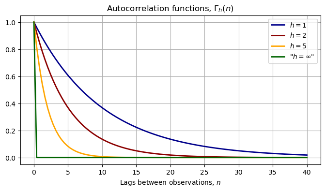
The following figure illustrates how the dependence between the observations is related to the sampling frequency
For any given \(h\), the autocorrelation converges to zero as we increase the distance – \(n\)– between the observations. This represents the “weak dependence” of the \(X\) process.
Moreover, for a fixed lag length, \(n\), the dependence vanishes as the sampling frequency goes to infinity. In fact, letting \(h\) go to \(\infty\) gives back the case of IID data.
μ = .0
κ = .1
σ = .5
var_uncond = σ**2 / (2 * κ)

n_grid = np.linspace(0, 40, 100)
autocorr_h1 = np.exp(-κ * n_grid * 1)
autocorr_h2 = np.exp(-κ * n_grid * 2)
autocorr_h5 = np.exp(-κ * n_grid * 5)
autocorr_h1000 = np.exp(-κ * n_grid * 1e8)

fig, ax = plt.subplots(figsize=(8, 4))
ax.plot(n_grid, autocorr_h1, label=r'$h=1$', c='darkblue', lw=2)
ax.plot(n_grid, autocorr_h2, label=r'$h=2$', c='darkred', lw=2)
ax.plot(n_grid, autocorr_h5, label=r'$h=5$', c='orange', lw=2)
ax.plot(n_grid, autocorr_h1000, label=r'"$h=\infty$"', c='darkgreen', lw=2)
ax.legend()
ax.grid()
ax.set(title=r'Autocorrelation functions, $\Gamma_h(n)$',
       xlabel=r'Lags between observations, $n$')
plt.show()
44.15. Frequency and the mean estimator#
Consider again the AR(1) process generated by discrete sampling with frequency \(h\). Assume that we have a sample of size \(N\) and we would like to estimate the unconditional mean – in our case the true mean is \(\mu\).
Again, the sample average is an unbiased estimator of the unconditional mean
The variance of the sample mean is given by
It is explicit in the above equation that time dependence in the data inflates the variance of the mean estimator through the covariance terms.
Moreover, as we can see, a higher sampling frequency—smaller \(h\)—makes all the covariance terms larger, everything else being fixed.
This implies a relatively slower rate of convergence of the sample average for high-frequency data.
Intuitively, stronger dependence across observations for high-frequency data reduces the “information content” of each observation relative to the IID case.
We can upper bound the variance term in the following way
Asymptotically, the term \(\exp(-\kappa h)^{N-1}\) vanishes and the dependence in the data inflates the benchmark IID variance by a factor of
This long run factor is larger the higher is the frequency (the smaller is \(h\)).
Therefore, we expect the asymptotic relative MSEs, \(B\), to change with time-dependent data. We just saw that the mean estimator’s rate is roughly changing by a factor of
Unfortunately, the variance estimator’s MSE is harder to derive.
Nonetheless, we can approximate it by using (large sample) simulations, thus getting an idea about how the asymptotic relative MSEs changes in the sampling frequency \(h\) relative to the IID case that we compute in closed form.
@jit
def sample_generator(h, N, M):
    ϕ = (1 - np.exp(-κ * h)) * μ
    ρ = np.exp(-κ * h)
    s = σ**2 * (1 - np.exp(-2 * κ * h)) / (2 * κ)

    mean_uncond = μ
    std_uncond = np.sqrt(σ**2 / (2 * κ))

    ε_path = np.random.normal(0, np.sqrt(s), (M, N))

    y_path = np.zeros((M, N + 1))
    y_path[:, 0] = np.random.normal(mean_uncond, std_uncond, M)

    for i in range(N):
        y_path[:, i + 1] = ϕ + ρ * y_path[:, i] + ε_path[:, i]

    return y_path
# Generate large sample for different frequencies
N_app, M_app = 1000, 30000        # Sample size, number of simulations
h_grid = np.linspace(.1, 80, 30)

var_est_store = []
mean_est_store = []
labels = []

for h in h_grid:
    labels.append(h)
    sample = sample_generator(h, N_app, M_app)
    mean_est_store.append(np.mean(sample, 1))
    var_est_store.append(np.var(sample, 1))

var_est_store = np.array(var_est_store)
mean_est_store = np.array(mean_est_store)

# Save mse of estimators
mse_mean = np.var(mean_est_store, 1) + (np.mean(mean_est_store, 1) - μ)**2
mse_var = np.var(var_est_store, 1) \
          + (np.mean(var_est_store, 1) - var_uncond)**2

benchmark_rate = 2 * var_uncond       # IID case

# Relative MSE for large samples
rate_h = mse_var / mse_mean

fig, ax = plt.subplots(figsize=(8, 5))
ax.plot(h_grid, rate_h, c='darkblue', lw=2,
        label=r'large sample relative MSE, $B(h)$')
ax.axhline(benchmark_rate, c='k', ls='--', label=r'IID benchmark')
ax.set_title('Relative MSE for large samples as a function of sampling \
              frequency \n MSE($S_N$) relative to MSE($\\bar X_N$)')
ax.set_xlabel('Sampling frequency, $h$')
ax.legend()
plt.show()
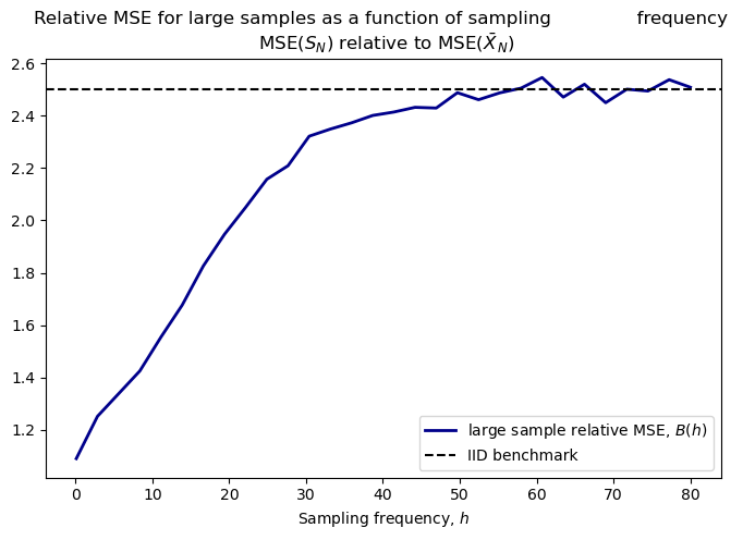
The above figure illustrates the relationship between the asymptotic relative MSEs and the sampling frequency
We can see that with low-frequency data – large values of \(h\) – the ratio of asymptotic rates approaches the IID case.
As \(h\) gets smaller – the higher the frequency – the relative performance of the variance estimator is better in the sense that the ratio of asymptotic rates gets smaller. That is, as the time dependence gets more pronounced, the rate of convergence of the mean estimator’s MSE deteriorates more than that of the variance estimator.