27. Robust Markov Perfect Equilibrium#

In addition to what’s in Anaconda, this lecture will need the following libraries:

!pip install --upgrade quantecon

27.1. Overview#

This lecture describes a Markov perfect equilibrium with robust agents.

We focus on special settings with

two players
quadratic payoff functions
linear transition rules for the state vector

These specifications simplify calculations and allow us to give a simple example that illustrates basic forces.

This lecture is based on ideas described in chapter 15 of [Hansen and Sargent, 2008] and in Markov perfect equilibrium and Robustness.

Let’s start with some standard imports:

import numpy as np
import quantecon as qe
from scipy.linalg import solve
import matplotlib.pyplot as plt

27.1.1. Basic Setup#

Decisions of two agents affect the motion of a state vector that appears as an argument of payoff functions of both agents.

As described in Markov perfect equilibrium, when decision-makers have no concerns about the robustness of their decision rules to misspecifications of the state dynamics, a Markov perfect equilibrium can be computed via backward recursion on two sets of equations

a pair of Bellman equations, one for each agent.
a pair of equations that express linear decision rules for each agent as functions of that agent’s continuation value function as well as parameters of preferences and state transition matrices.

This lecture shows how a similar equilibrium concept and similar computational procedures apply when we impute concerns about robustness to both decision-makers.

A Markov perfect equilibrium with robust agents will be characterized by

a pair of Bellman equations, one for each agent.
a pair of equations that express linear decision rules for each agent as functions of that agent’s continuation value function as well as parameters of preferences and state transition matrices.
a pair of equations that express linear decision rules for worst-case shocks for each agent as functions of that agent’s continuation value function as well as parameters of preferences and state transition matrices.

Below, we’ll construct a robust firms version of the classic duopoly model with adjustment costs analyzed in Markov perfect equilibrium.

27.2. Linear Markov Perfect Equilibria with Robust Agents#

As we saw in Markov perfect equilibrium, the study of Markov perfect equilibria in dynamic games with two players leads us to an interrelated pair of Bellman equations.

In linear quadratic dynamic games, these “stacked Bellman equations” become “stacked Riccati equations” with a tractable mathematical structure.

27.2.1. Modified Coupled Linear Regulator Problems#

We consider a general linear quadratic regulator game with two players, each of whom fears model misspecifications.

We often call the players agents.

The agents share a common baseline model for the transition dynamics of the state vector

this is a counterpart of a ‘rational expectations’ assumption of shared beliefs

But now one or more agents doubt that the baseline model is correctly specified.

The agents express the possibility that their baseline specification is incorrect by adding a contribution \(C v_{it}\) to the time \(t\) transition law for the state

\(C\) is the usual volatility matrix that appears in stochastic versions of optimal linear regulator problems.
\(v_{it}\) is a possibly history-dependent vector of distortions to the dynamics of the state that agent \(i\) uses to represent misspecification of the original model.

For convenience, we’ll start with a finite horizon formulation, where \(t_0\) is the initial date and \(t_1\) is the common terminal date.

Player \(i\) takes a sequence \(\{u_{-it}\}\) as given and chooses a sequence \(\{u_{it}\}\) to minimize and \(\{v_{it}\}\) to maximize

(27.1)#\[\sum_{t=t_0}^{t_1 - 1} \beta^{t - t_0} \left\{ x_t' R_i x_t + u_{it}' Q_i u_{it} + u_{-it}' S_i u_{-it} + 2 x_t' W_i u_{it} + 2 u_{-it}' M_i u_{it} - \theta_i v_{it}' v_{it} \right\}\]

while thinking that the state evolves according to

(27.2)#\[x_{t+1} = A x_t + B_1 u_{1t} + B_2 u_{2t} + C v_{it}\]

Here

\(x_t\) is an \(n \times 1\) state vector, \(u_{it}\) is a \(k_i \times 1\) vector of controls for player \(i\), and
\(v_{it}\) is an \(h \times 1\) vector of distortions to the state dynamics that concern player \(i\)
\(R_i\) is \(n \times n\)
\(S_i\) is \(k_{-i} \times k_{-i}\)
\(Q_i\) is \(k_i \times k_i\)
\(W_i\) is \(n \times k_i\)
\(M_i\) is \(k_{-i} \times k_i\)
\(A\) is \(n \times n\)
\(B_i\) is \(n \times k_i\)
\(C\) is \(n \times h\)
\(\theta_i \in [\underline \theta_i, +\infty]\) is a scalar multiplier parameter of player \(i\)

If \(\theta_i = + \infty\), player \(i\) completely trusts the baseline model.

If \(\theta_i < _\infty\), player \(i\) suspects that some other unspecified model actually governs the transition dynamics.

The term \(\theta_i v_{it}' v_{it}\) is a time \(t\) contribution to an entropy penalty that an (imaginary) loss-maximizing agent inside agent \(i\)’s mind charges for distorting the law of motion in a way that harms agent \(i\).

the imaginary loss-maximizing agent helps the loss-minimizing agent by helping him construct bounds on the behavior of his decision rule over a large set of alternative models of state transition dynamics.

27.2.2. Computing Equilibrium#

We formulate a linear robust Markov perfect equilibrium as follows.

Player \(i\) employs linear decision rules \(u_{it} = - F_{it} x_t\), where \(F_{it}\) is a \(k_i \times n\) matrix.

Player \(i\)’s malevolent alter ego employs decision rules \(v_{it} = K_{it} x_t\) where \(K_{it}\) is an \(h \times n\) matrix.

A robust Markov perfect equilibrium is a pair of sequences \(\{F_{1t}, F_{2t}\}\) and a pair of sequences \(\{K_{1t}, K_{2t}\}\) over \(t = t_0, \ldots, t_1 - 1\) that satisfy

\(\{F_{1t}, K_{1t}\}\) solves player 1’s robust decision problem, taking \(\{F_{2t}\}\) as given, and
\(\{F_{2t}, K_{2t}\}\) solves player 2’s robust decision problem, taking \(\{F_{1t}\}\) as given.

If we substitute \(u_{2t} = - F_{2t} x_t\) into (27.1) and (27.2), then player 1’s problem becomes minimization-maximization of

(27.3)#\[\sum_{t=t_0}^{t_1 - 1} \beta^{t - t_0} \left\{ x_t' \Pi_{1t} x_t + u_{1t}' Q_1 u_{1t} + 2 u_{1t}' \Gamma_{1t} x_t - \theta_1 v_{1t}' v_{1t} \right\}\]

subject to

(27.4)#\[x_{t+1} = \Lambda_{1t} x_t + B_1 u_{1t} + C v_{1t}\]

where

\(\Lambda_{it} := A - B_{-i} F_{-it}\)
\(\Pi_{it} := R_i + F_{-it}' S_i F_{-it}\)
\(\Gamma_{it} := W_i' - M_i' F_{-it}\)

This is an LQ robust dynamic programming problem of the type studied in the Robustness lecture, which can be solved by working backward.

Maximization with respect to distortion \(v_{1t}\) leads to the following version of the \(\mathcal D\) operator from the Robustness lecture, namely

(27.5)#\[\mathcal D_1(P) := P + PC (\theta_1 I - C' P C)^{-1} C' P\]

The matrix \(F_{1t}\) in the policy rule \(u_{1t} = - F_{1t} x_t\) that solves agent 1’s problem satisfies

(27.6)#\[F_{1t} = (Q_1 + \beta B_1' {\mathcal D}_1( P_{1t+1}) B_1)^{-1} (\beta B_1' {\mathcal D}_1( P_{1t+1}) \Lambda_{1t} + \Gamma_{1t})\]

where \(P_{1t}\) solves the matrix Riccati difference equation

(27.7)#\[\begin{split}P_{1t} = \Pi_{1t} - (\beta B_1' {\mathcal D}_1(P_{1t+1}) \Lambda_{1t} + \Gamma_{1t})' (Q_1 + \beta B_1' {\mathcal D}_1( P_{1t+1}) B_1)^{-1} (\beta B_1' {\mathcal D}_1(P_{1t+1}) \Lambda_{1t} + \Gamma_{1t}) + \\ \beta \Lambda_{1t}' {\mathcal D}_1(P_{1t+1}) \Lambda_{1t}\end{split}\]

Similarly, the policy that solves player 2’s problem is

(27.8)#\[F_{2t} = (Q_2 + \beta B_2' {\mathcal D}_2( P_{2t+1} ) B_2)^{-1} (\beta B_2' {\mathcal D}_2 (P_{2t+1}) \Lambda_{2t} + \Gamma_{2t})\]

where \(P_{2t}\) solves

(27.9)#\[\begin{split}P_{2t} = \Pi_{2t} - (\beta B_2' {\mathcal D}_2 ( P_{2t+1}) \Lambda_{2t} + \Gamma_{2t})' (Q_2 + \beta B_2' {\mathcal D}_2 ( P_{2t+1}) B_2)^{-1}(\beta B_2' {\mathcal D}_2 ( P_{2t+1}) \Lambda_{2t} + \Gamma_{2t}) + \\ \beta \Lambda_{2t}' {\mathcal D}_2 ( P_{2t+1}) \Lambda_{2t}\end{split}\]

Here in all cases \(t = t_0, \ldots, t_1 - 1\) and the terminal conditions are \(P_{it_1} = 0\).

The solution procedure is to use equations (27.6), (27.7), (27.8), and (27.9), and “work backwards” from time \(t_1 - 1\).

Since we’re working backwards, \(P_{1t+1}\) and \(P_{2t+1}\) are taken as given at each stage.

Moreover, since

some terms on the right-hand side of (27.6) contain \(F_{2t}\)
some terms on the right-hand side of (27.8) contain \(F_{1t}\)

we need to solve these \(k_1 + k_2\) equations simultaneously.

27.2.3. Key Insight#

As in Markov perfect equilibrium, a key insight here is that equations (27.6) and (27.8) are linear in \(F_{1t}\) and \(F_{2t}\).

After these equations have been solved, we can take \(F_{it}\) and solve for \(P_{it}\) in (27.7) and (27.9).

Notice how \(j\)’s control law \(F_{jt}\) is a function of \(\{F_{is}, s \geq t, i \neq j \}\).

Thus, agent \(i\)’s choice of \(\{F_{it}; t = t_0, \ldots, t_1 - 1\}\) influences agent \(j\)’s choice of control laws.

However, in the Markov perfect equilibrium of this game, each agent is assumed to ignore the influence that his choice exerts on the other agent’s choice.

After these equations have been solved, we can also deduce associated sequences of worst-case shocks.

27.2.4. Worst-case Shocks#

For agent \(i\) the maximizing or worst-case shock \(v_{it}\) is

\[ v_{it} = K_{it} x_t \]

where

\[ K_{it} = \theta_i^{-1} (I - \theta_i^{-1} C' P_{i,t+1} C)^{-1} C' P_{i,t+1} (A - B_1 F_{it} - B_2 F_{2t}) \]

27.2.5. Infinite Horizon#

We often want to compute the solutions of such games for infinite horizons, in the hope that the decision rules \(F_{it}\) settle down to be time-invariant as \(t_1 \rightarrow +\infty\).

In practice, we usually fix \(t_1\) and compute the equilibrium of an infinite horizon game by driving \(t_0 \rightarrow - \infty\).

This is the approach we adopt in the next section.

27.2.6. Implementation#

We use the function nnash_robust to compute a Markov perfect equilibrium of the infinite horizon linear quadratic dynamic game with robust planers in the manner described above.

27.3. Application#

27.3.1. A Duopoly Model#

Without concerns for robustness, the model is identical to the duopoly model from the Markov perfect equilibrium lecture.

To begin, we briefly review the structure of that model.

Two firms are the only producers of a good the demand for which is governed by a linear inverse demand function

(27.10)#\[p = a_0 - a_1 (q_1 + q_2)\]

Here \(p = p_t\) is the price of the good, \(q_i = q_{it}\) is the output of firm \(i=1,2\) at time \(t\) and \(a_0 > 0, a_1 >0\).

In (27.10) and what follows,

the time subscript is suppressed when possible to simplify notation
\(\hat x\) denotes a next period value of variable \(x\)

Each firm recognizes that its output affects total output and therefore the market price.

The one-period payoff function of firm \(i\) is price times quantity minus adjustment costs:

(27.11)#\[\pi_i = p q_i - \gamma (\hat q_i - q_i)^2, \quad \gamma > 0 ,\]

Substituting the inverse demand curve (27.10) into (27.11) lets us express the one-period payoff as

(27.12)#\[\pi_i(q_i, q_{-i}, \hat q_i) = a_0 q_i - a_1 q_i^2 - a_1 q_i q_{-i} - \gamma (\hat q_i - q_i)^2 ,\]

where \(q_{-i}\) denotes the output of the firm other than \(i\).

The objective of the firm is to maximize \(\sum_{t=0}^\infty \beta^t \pi_{it}\).

Firm \(i\) chooses a decision rule that sets next period quantity \(\hat q_i\) as a function \(f_i\) of the current state \((q_i, q_{-i})\).

This completes our review of the duopoly model without concerns for robustness.

Now we activate robustness concerns of both firms.

To map a robust version of the duopoly model into coupled robust linear-quadratic dynamic programming problems, we again define the state and controls as

\[\begin{split} x_t := \begin{bmatrix} 1 \\ q_{1t} \\ q_{2t} \end{bmatrix} \quad \text{and} \quad u_{it} := q_{i,t+1} - q_{it}, \quad i=1,2 \end{split}\]

If we write

\[ x_t' R_i x_t + u_{it}' Q_i u_{it} \]

where \(Q_1 = Q_2 = \gamma\),

\[\begin{split} R_1 := \begin{bmatrix} 0 & -\frac{a_0}{2} & 0 \\ -\frac{a_0}{2} & a_1 & \frac{a_1}{2} \\ 0 & \frac{a_1}{2} & 0 \end{bmatrix} \quad \text{and} \quad R_2 := \begin{bmatrix} 0 & 0 & -\frac{a_0}{2} \\ 0 & 0 & \frac{a_1}{2} \\ -\frac{a_0}{2} & \frac{a_1}{2} & a_1 \end{bmatrix} \end{split}\]

then we recover the one-period payoffs (27.11) for the two firms in the duopoly model.

The law of motion for the state \(x_t\) is \(x_{t+1} = A x_t + B_1 u_{1t} + B_2 u_{2t}\) where

\[\begin{split} A := \begin{bmatrix} 1 & 0 & 0 \\ 0 & 1 & 0 \\ 0 & 0 & 1 \end{bmatrix}, \quad B_1 := \begin{bmatrix} 0 \\ 1 \\ 0 \end{bmatrix}, \quad B_2 := \begin{bmatrix} 0 \\ 0 \\ 1 \end{bmatrix} \end{split}\]

A robust decision rule of firm \(i\) will take the form \(u_{it} = - F_i x_t\), inducing the following closed-loop system for the evolution of \(x\) in the Markov perfect equilibrium:

(27.13)#\[x_{t+1} = (A - B_1 F_1 -B_1 F_2 ) x_t\]

27.3.2. Parameters and Solution#

Consider the duopoly model with parameter values of:

\(a_0 = 10\)
\(a_1 = 2\)
\(\beta = 0.96\)
\(\gamma = 12\)

From these, we computed the infinite horizon MPE without robustness using the code

import numpy as np
import quantecon as qe

# Parameters
a0 = 10.0
a1 = 2.0
β = 0.96
γ = 12.0

# In LQ form
A = np.eye(3)
B1 = np.array([[0.], [1.], [0.]])
B2 = np.array([[0.], [0.], [1.]])


R1 = [[      0.,     -a0 / 2,          0.],
      [-a0 / 2.,          a1,     a1 / 2.],
      [       0,     a1 / 2.,          0.]]

R2 = [[     0.,           0.,      -a0 / 2],
      [     0.,           0.,      a1 / 2.],
      [-a0 / 2,      a1 / 2.,           a1]]

Q1 = Q2 = γ
S1 = S2 = W1 = W2 = M1 = M2 = 0.0

# Solve using QE's nnash function
F1, F2, P1, P2 = qe.nnash(A, B1, B2, R1, R2, Q1, 
                          Q2, S1, S2, W1, W2, M1, 
                          M2, beta=β)

# Display policies
print("Computed policies for firm 1 and firm 2:\n")
print(f"F1 = {F1}")
print(f"F2 = {F2}")
print("\n")

Computed policies for firm 1 and firm 2:

F1 = [[-0.66846615  0.29512482  0.07584666]]
F2 = [[-0.66846615  0.07584666  0.29512482]]

27.3.2.1. Markov Perfect Equilibrium with Robustness#

We add robustness concerns to the Markov Perfect Equilibrium model by extending the function qe.nnash (link) into a robustness version by adding the maximization operator \(\mathcal D(P)\) into the backward induction.

The MPE with robustness function is nnash_robust.

The function’s code is as follows

def nnash_robust(A, C, B1, B2, R1, R2, Q1, Q2, S1, S2, W1, W2, M1, M2,
                 θ1, θ2, beta=1.0, tol=1e-8, max_iter=1000):

    """
    Compute the limit of a Nash linear quadratic dynamic game with
    robustness concern.

    In this problem, player i minimizes
    .. math::
        \sum_{t=0}^{\infty}
        \left\{
            x_t' r_i x_t + 2 x_t' w_i
            u_{it} +u_{it}' q_i u_{it} + u_{jt}' s_i u_{jt} + 2 u_{jt}'
            m_i u_{it}
        \right\}
    subject to the law of motion
    .. math::
        x_{it+1} = A x_t + b_1 u_{1t} + b_2 u_{2t} + C w_{it+1}
    and a perceived control law :math:`u_j(t) = - f_j x_t` for the other
    player.

    The player i also concerns about the model misspecification,
    and maximizes
    .. math::
        \sum_{t=0}^{\infty}
        \left\{
            \beta^{t+1} \theta_{i} w_{it+1}'w_{it+1}
        \right\}

    The solution computed in this routine is the :math:`f_i` and
    :math:`P_i` of the associated double optimal linear regulator
    problem.

    Parameters
    ----------
    A : scalar(float) or array_like(float)
        Corresponds to the MPE equations, should be of size (n, n)
    C : scalar(float) or array_like(float)
        As above, size (n, c), c is the size of w
    B1 : scalar(float) or array_like(float)
        As above, size (n, k_1)
    B2 : scalar(float) or array_like(float)
        As above, size (n, k_2)
    R1 : scalar(float) or array_like(float)
        As above, size (n, n)
    R2 : scalar(float) or array_like(float)
        As above, size (n, n)
    Q1 : scalar(float) or array_like(float)
        As above, size (k_1, k_1)
    Q2 : scalar(float) or array_like(float)
        As above, size (k_2, k_2)
    S1 : scalar(float) or array_like(float)
        As above, size (k_1, k_1)
    S2 : scalar(float) or array_like(float)
        As above, size (k_2, k_2)
    W1 : scalar(float) or array_like(float)
        As above, size (n, k_1)
    W2 : scalar(float) or array_like(float)
        As above, size (n, k_2)
    M1 : scalar(float) or array_like(float)
        As above, size (k_2, k_1)
    M2 : scalar(float) or array_like(float)
        As above, size (k_1, k_2)
    θ1 : scalar(float)
            Robustness parameter of player 1
    θ2 : scalar(float)
            Robustness parameter of player 2
    beta : scalar(float), optional(default=1.0)
          Discount factor
    tol : scalar(float), optional(default=1e-8)
         This is the tolerance level for convergence
    max_iter : scalar(int), optional(default=1000)
        This is the maximum number of iterations allowed

    Returns
    -------
    F1 : array_like, dtype=float, shape=(k_1, n)
        Feedback law for agent 1
    F2 : array_like, dtype=float, shape=(k_2, n)
        Feedback law for agent 2
    P1 : array_like, dtype=float, shape=(n, n)
        The steady-state solution to the associated discrete matrix
        Riccati equation for agent 1
    P2 : array_like, dtype=float, shape=(n, n)
        The steady-state solution to the associated discrete matrix
        Riccati equation for agent 2
    """

    # Unload parameters and make sure everything is a matrix
    params = A, C, B1, B2, R1, R2, Q1, Q2, S1, S2, W1, W2, M1, M2
    params = map(np.asmatrix, params)
    A, C, B1, B2, R1, R2, Q1, Q2, S1, S2, W1, W2, M1, M2 = params


    # Multiply A, B1, B2 by sqrt(β) to enforce discounting
    A, B1, B2 = [np.sqrt(β) * x for x in (A, B1, B2)]

    # Initial values
    n = A.shape[0]
    k_1 = B1.shape[1]
    k_2 = B2.shape[1]

    v1 = np.eye(k_1)
    v2 = np.eye(k_2)
    P1 = np.eye(n) * 1e-5
    P2 = np.eye(n) * 1e-5
    F1 = np.random.randn(k_1, n)
    F2 = np.random.randn(k_2, n)


    for it in range(max_iter):
        # Update
        F10 = F1
        F20 = F2

        I = np.eye(C.shape[1])

        # D1(P1)
        # Note: INV1 may not be solved if the matrix is singular
        INV1 = solve(θ1 * I - C.T @ P1 @ C, I)
        D1P1 =  P1 + P1 @ C @ INV1 @ C.T @ P1

        # D2(P2)
        # Note: INV2 may not be solved if the matrix is singular
        INV2 = solve(θ2 * I - C.T @ P2 @ C, I)
        D2P2 =  P2 + P2 @ C @ INV2 @ C.T @ P2

        G2 = solve(Q2 + B2.T @ D2P2 @ B2, v2)
        G1 = solve(Q1 + B1.T @ D1P1 @ B1, v1)
        H2 = G2 @ B2.T @ D2P2
        H1 = G1 @ B1.T @ D1P1

        # Break up the computation of F1, F2
        F1_left = v1 - (H1 @ B2 + G1 @ M1.T) @ (H2 @ B1 + G2 @ M2.T)
        F1_right = H1 @ A + G1 @ W1.T - \
                   (H1 @ B2 + G1 @ M1.T) @ (H2 @ A + G2 @ W2.T)
        F1 = solve(F1_left, F1_right)
        F2 = H2 @ A + G2 @ W2.T - (H2 @ B1 + G2 @ M2.T) @ F1

        Λ1 = A - B2 @ F2
        Λ2 = A - B1 @ F1
        Π1 = R1 + F2.T @ S1 @ F2
        Π2 = R2 + F1.T @ S2 @ F1
        Γ1 = W1.T - M1.T @ F2
        Γ2 = W2.T - M2.T @ F1

        # Compute P1 and P2
        P1 = Π1 - (B1.T @ D1P1 @ Λ1 + Γ1).T @ F1 + \
             Λ1.T @ D1P1 @ Λ1
        P2 = Π2 - (B2.T @ D2P2 @ Λ2 + Γ2).T @ F2 + \
             Λ2.T @ D2P2 @ Λ2

        dd = np.max(np.abs(F10 - F1)) + np.max(np.abs(F20 - F2))

        if dd < tol:  # success!
            break

    else:
        raise ValueError(f'No convergence: Iteration limit of {max_iter} \
            reached in nnash')

    return F1, F2, P1, P2

27.3.3. Some Details#

Firm \(i\) wants to minimize

\[ \sum_{t=t_0}^{t_1 - 1} \beta^{t - t_0} \left\{ x_t' R_i x_t + u_{it}' Q_i u_{it} + u_{-it}' S_i u_{-it} + 2 x_t' W_i u_{it} + 2 u_{-it}' M_i u_{it} \right\} \]

where

\[\begin{split} \begin{split} x_t := \begin{bmatrix} 1 \\ q_{1t} \\ q_{2t} \end{bmatrix} \quad \text{and} \quad u_{it} := q_{i,t+1} - q_{it}, \quad i=1,2 \end{split} \end{split}\]

and

\[\begin{split} \begin{split} R_1 := \begin{bmatrix} 0 & -\frac{a_0}{2} & 0 \\ -\frac{a_0}{2} & a_1 & \frac{a_1}{2} \\ 0 & \frac{a_1}{2} & 0 \end{bmatrix} \text{,} \quad R_2 := \begin{bmatrix} 0 & 0 & -\frac{a_0}{2} \\ 0 & 0 & \frac{a_1}{2} \\ -\frac{a_0}{2} & \frac{a_1}{2} & a_1 \end{bmatrix} \text{,} \quad Q_1 = Q_2 = \gamma \text{,} \quad S_1 = S_2 = 0 \text{,} \quad W_1 = W_2 = 0 \text{,} \quad M_1 = M_2 = 0 \end{split} \end{split}\]

The parameters of the duopoly model are:

\(a_0 = 10\)
\(a_1 = 2\)
\(\beta = 0.96\)
\(\gamma = 12\)

# Parameters
a0 = 10.0
a1 = 2.0
β = 0.96
γ = 12.0


# In LQ form
A = np.eye(3)
B1 = np.array([[0.], [1.], [0.]])
B2 = np.array([[0.], [0.], [1.]])


R1 = [[      0.,     -a0 / 2,          0.],
      [-a0 / 2.,          a1,     a1 / 2.],
      [       0,     a1 / 2.,          0.]]

R2 = [[     0.,           0.,      -a0 / 2],
      [     0.,           0.,      a1 / 2.],
      [-a0 / 2,      a1 / 2.,           a1]]

Q1 = Q2 = γ
S1 = S2 = W1 = W2 = M1 = M2 = 0.0

27.3.3.1. Consistency Check#

We first conduct a comparison test to check if nnash_robust agrees with qe.nnash in the non-robustness case in which each \(\theta_i \approx +\infty\)

# Solve using QE's nnash function
F1, F2, P1, P2 = qe.nnash(A, B1, B2, R1, R2, Q1,
                          Q2, S1, S2, W1, W2, M1,
                          M2, beta=β)

# Solve using nnash_robust
F1r, F2r, P1r, P2r = nnash_robust(A, np.zeros((3, 1)), B1, B2, R1, R2, Q1,
                                  Q2, S1, S2, W1, W2, M1, M2, 1e-10,
                                  1e-10, beta=β)

print('F1 and F1r should be the same: ', np.allclose(F1, F1r))
print('F2 and F2r should be the same: ', np.allclose(F1, F1r))
print('P1 and P1r should be the same: ', np.allclose(P1, P1r))
print('P2 and P2r should be the same: ', np.allclose(P1, P1r))

F1 and F1r should be the same:  True
F2 and F2r should be the same:  True
P1 and P1r should be the same:  True
P2 and P2r should be the same:  True

We can see that the results are consistent across the two functions.

27.3.3.2. Comparative Dynamics under Baseline Transition Dynamics#

We want to compare the dynamics of price and output under the baseline MPE model with those under the baseline model under the robust decision rules within the robust MPE.

This means that we simulate the state dynamics under the MPE equilibrium closed-loop transition matrix

\[ A^o = A - B_1 F_1 - B_2 F_2 \]

where \(F_1\) and \(F_2\) are the firms’ robust decision rules within the robust markov_perfect equilibrium

by simulating under the baseline model transition dynamics and the robust MPE rules we are in assuming that at the end of the day firms’ concerns about misspecification of the baseline model do not materialize.
a short way of saying this is that misspecification fears are all ‘just in the minds’ of the firms.
simulating under the baseline model is a common practice in the literature.
note that some assumption about the model that actually governs the data has to be made in order to create a simulation.
later we will describe the (erroneous) beliefs of the two firms that justify their robust decisions as best responses to transition laws that are distorted relative to the baseline model.

After simulating \(x_t\) under the baseline transition dynamics and robust decision rules \(F_i, i = 1, 2\), we extract and plot industry output \(q_t=q_{1t}+q_{2t}\) and price \(p_t = a_0 − a_1 q_t\).

Here we set the robustness and volatility matrix parameters as follows:

\(\theta_1 = 0.02\)
\(\theta_2 = 0.04\)
\(C = \begin{pmatrix} 0 \\ 0.01 \\ 0.01 \end{pmatrix}\)

Because we have set \(\theta_1 < \theta_2 < + \infty\) we know that

both firms fear that the baseline specification of the state transition dynamics are incorrect.
firm \(1\) fears misspecification more than firm \(2\).

# Robustness parameters and matrix
C = np.asmatrix([[0], [0.01], [0.01]])
θ1 = 0.02
θ2 = 0.04
n = 20


# Solve using nnash_robust
F1r, F2r, P1r, P2r = nnash_robust(A, C, B1, B2, R1, R2, Q1,
                                  Q2, S1, S2, W1, W2, M1, M2,
                                  θ1, θ2, beta=β)



# MPE output and price
AF = A - B1 @ F1 - B2 @ F2
x = np.empty((3, n))
x[:, 0] = 1, 1, 1
for t in range(n - 1):
    x[:, t + 1] = AF @ x[:, t]
q1 = x[1, :]
q2 = x[2, :]
q = q1 + q2       # Total output, MPE
p = a0 - a1 * q   # Price, MPE


# RMPE output and price
AO = A - B1 @ F1r - B2 @ F2r
xr = np.empty((3, n))
xr[:, 0] = 1, 1, 1
for t in range(n - 1):
    xr[:, t+1] = AO @ xr[:, t]
qr1 = xr[1, :]
qr2 = xr[2, :]
qr = qr1 + qr2      # Total output, RMPE
pr = a0 - a1 * qr   # Price, RMPE

# RMPE heterogeneous beliefs output and price
I = np.eye(C.shape[1])
INV1 = solve(θ1 * I - C.T @ P1 @ C, I)
K1 =  P1 @ C @ INV1 @ C.T @ P1 @ AO
AOCK1 = AO + C.T @ K1

INV2 = solve(θ2 * I - C.T @ P2 @ C, I)
K2 =  P2 @ C @ INV2 @ C.T @ P2 @ AO
AOCK2 = AO + C.T @ K2
xrp1 = np.empty((3, n))
xrp2 = np.empty((3, n))
xrp1[:, 0] = 1, 1, 1
xrp2[:, 0] = 1, 1, 1
for t in range(n - 1):
    xrp1[:, t + 1] = AOCK1 @ xrp1[:, t]
    xrp2[:, t + 1] = AOCK2 @ xrp2[:, t]
qrp11 = xrp1[1, :]
qrp12 = xrp1[2, :]
qrp21 = xrp2[1, :]
qrp22 = xrp2[2, :]
qrp1 = qrp11 + qrp12       # Total output, RMPE from player 1's belief
qrp2 = qrp21 + qrp22       # Total output, RMPE from player 2's belief
prp1 = a0 - a1 * qrp1      # Price, RMPE from player 1's belief
prp2 = a0 - a1 * qrp2      # Price, RMPE from player 2's belief

The following code prepares graphs that compare market-wide output \(q_{1t} + q_{2t}\) and the price of the good \(p_t\) under equilibrium decision rules \(F_i, i = 1, 2\) from an ordinary Markov perfect equilibrium and the decision rules under a Markov perfect equilibrium with robust firms with multiplier parameters \(\theta_i, i = 1,2\) set as described above.

Both industry output and price are under the transition dynamics associated with the baseline model; only the decision rules \(F_i\) differ across the two equilibrium objects presented.

fig, axes = plt.subplots(2, 1, figsize=(9, 9))

ax = axes[0]
ax.plot(q, 'g-', lw=2, alpha=0.75, label='MPE output')
ax.plot(qr, 'm-', lw=2, alpha=0.75, label='RMPE output')
ax.set(ylabel="output", xlabel="time", ylim=(2, 4))
ax.legend(loc='upper left', frameon=0)

ax = axes[1]
ax.plot(p, 'g-', lw=2, alpha=0.75, label='MPE price')
ax.plot(pr, 'm-', lw=2, alpha=0.75, label='RMPE price')
ax.set(ylabel="price", xlabel="time")
ax.legend(loc='upper right', frameon=0)
plt.show()

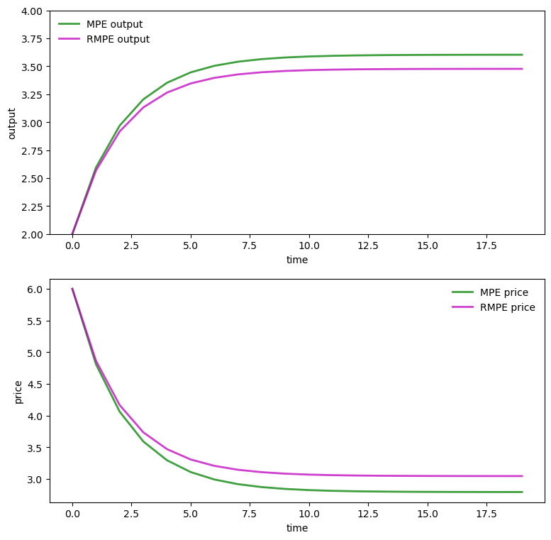
_images/a638c67810bde3919fa21c6511deb46563da1f2a3ea623b32bffc03c53408e11.png

Under the dynamics associated with the baseline model, the price path is higher with the Markov perfect equilibrium robust decision rules than it is with decision rules for the ordinary Markov perfect equilibrium.

So is the industry output path.

To dig a little beneath the forces driving these outcomes, we want to plot \(q_{1t}\) and \(q_{2t}\) in the Markov perfect equilibrium with robust firms and to compare them with corresponding objects in the Markov perfect equilibrium without robust firms

fig, axes = plt.subplots(2, 1, figsize=(9, 9))

ax = axes[0]
ax.plot(q1, 'g-', lw=2, alpha=0.75, label='firm 1 MPE output')
ax.plot(qr1, 'b-', lw=2, alpha=0.75, label='firm 1 RMPE output')
ax.set(ylabel="output", xlabel="time", ylim=(1, 2))
ax.legend(loc='upper left', frameon=0)

ax = axes[1]
ax.plot(q2, 'g-', lw=2, alpha=0.75, label='firm 2 MPE output')
ax.plot(qr2, 'r-', lw=2, alpha=0.75, label='firm 2 RMPE output')
ax.set(ylabel="output", xlabel="time", ylim=(1, 2))
ax.legend(loc='upper left', frameon=0)
plt.show()

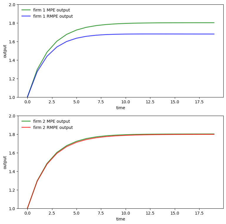
_images/ad3074e576cf40460c952b488dc75bfabbb5c59be76ec8a90af737767aca9aea.png

Evidently, firm 1’s output path is substantially lower when firms are robust firms while firm 2’s output path is virtually the same as it would be in an ordinary Markov perfect equilibrium with no robust firms.

Recall that we have set \(\theta_1 = .02\) and \(\theta_2 = .04\), so that firm 1 fears misspecification of the baseline model substantially more than does firm 2

but also please notice that firm \(2\)’s behavior in the Markov perfect equilibrium with robust firms responds to the decision rule \(F_1 x_t\) employed by firm \(1\).
thus it is something of a coincidence that its output is almost the same in the two equilibria.

Larger concerns about misspecification induce firm 1 to be more cautious than firm 2 in predicting market price and the output of the other firm.

To explore this, we study next how ex-post the two firms’ beliefs about state dynamics differ in the Markov perfect equilibrium with robust firms.

(by ex-post we mean after extremization of each firm’s intertemporal objective)

27.3.3.3. Heterogeneous Beliefs#

As before, let \(A^o = A - B\_1 F\_1^r - B\_2 F\_2^r\), where in a robust MPE, \(F_i^r\) is a robust decision rule for firm \(i\).

Worst-case forecasts of \(x_t\) starting from \(t=0\) differ between the two firms.

This means that worst-case forecasts of industry output \(q_{1t} + q_{2t}\) and price \(p_t\) also differ between the two firms.

To find these worst-case beliefs, we compute the following three “closed-loop” transition matrices

\(A^o\)
\(A^o + C K\_1\)
\(A^o + C K\_2\)

We call the first transition law, namely, \(A^o\), the baseline transition under firms’ robust decision rules.

We call the second and third worst-case transitions under robust decision rules for firms 1 and 2.

From \(\{x_t\}\) paths generated by each of these transition laws, we pull off the associated price and total output sequences.

The following code plots them

print('Baseline Robust transition matrix AO is: \n', np.round(AO, 3))
print('Player 1\'s worst-case transition matrix AOCK1 is: \n', \
np.round(AOCK1, 3))
print('Player 2\'s worst-case transition matrix AOCK2 is: \n', \
np.round(AOCK2, 3))

Baseline Robust transition matrix AO is: 
 [[ 1.     0.     0.   ]
 [ 0.666  0.682 -0.074]
 [ 0.671 -0.071  0.694]]
Player 1's worst-case transition matrix AOCK1 is: 
 [[ 0.998  0.002  0.   ]
 [ 0.664  0.685 -0.074]
 [ 0.669 -0.069  0.694]]
Player 2's worst-case transition matrix AOCK2 is: 
 [[ 0.999  0.     0.001]
 [ 0.665  0.683 -0.073]
 [ 0.67  -0.071  0.695]]

# == Plot == #
fig, axes = plt.subplots(2, 1, figsize=(9, 9))

ax = axes[0]
ax.plot(qrp1, 'b--', lw=2, alpha=0.75,
    label='RMPE worst-case belief output player 1')
ax.plot(qrp2, 'r:', lw=2, alpha=0.75,
    label='RMPE worst-case belief output player 2')
ax.plot(qr, 'm-', lw=2, alpha=0.75, label='RMPE output')
ax.set(ylabel="output", xlabel="time", ylim=(2, 4))
ax.legend(loc='upper left', frameon=0)

ax = axes[1]
ax.plot(prp1, 'b--', lw=2, alpha=0.75,
    label='RMPE worst-case belief price player 1')
ax.plot(prp2, 'r:', lw=2, alpha=0.75,
    label='RMPE worst-case belief price player 2')
ax.plot(pr, 'm-', lw=2, alpha=0.75, label='RMPE price')
ax.set(ylabel="price", xlabel="time")
ax.legend(loc='upper right', frameon=0)
plt.show()

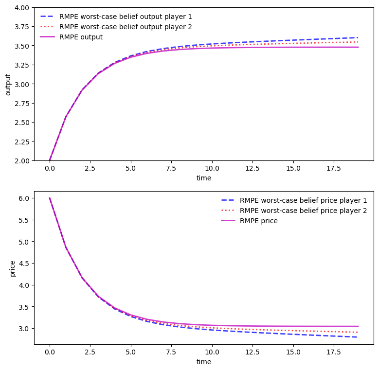
_images/f868f2e0267316bb0007038c5abc1410de5a22de6105a62d8d1b759d3fccde6d.png

We see from the above graph that under robustness concerns, player 1 and player 2 have heterogeneous beliefs about total output and the goods price even though they share the same baseline model and information

firm 1 thinks that total output will be higher and price lower than does firm 2
this leads firm 1 to produce less than firm 2

These beliefs justify (or rationalize) the Markov perfect equilibrium robust decision rules.

This means that the robust rules are the unique optimal rules (or best responses) to the indicated worst-case transition dynamics.

([Hansen and Sargent, 2008] discuss how this property of robust decision rules is connected to the concept of admissibility in Bayesian statistical decision theory)