41. Elementary Asset Pricing Theory#
41.1. Overview#
This lecture is about some implications of asset-pricing theories that are based on the equation \(E m R = 1,\) where \(R\) is the gross return on an asset, \(m\) is a stochastic discount factor, and \(E\) is a mathematical expectation with respect to a joint probability distribution of \(R\) and \(m\).
Instances of this equation occur in many models.
Note
Chapter 1 of [Ljungqvist and Sargent, 2018] describes the role that this equation plays in a diverse set of models in macroeconomics, monetary economics, and public finance.
We aim to convey insights about empirical implications of this equation brought out in the work of Lars Peter Hansen [Hansen and Richard, 1987] and Lars Peter Hansen and Ravi Jagannathan [Hansen and Jagannathan, 1991].
By following their footsteps, from that single equation we’ll derive
a mean-variance frontier
a single-factor model of excess returns
To do this, we use two ideas:
the equation \(E m R =1 \) that is implied by an application of a law of one price
a Cauchy-Schwartz inequality
In particular, we’ll apply a Cauchy-Schwartz inequality to a population linear least squares regression equation that is implied by \(E m R =1\).
We’ll also describe how practitioners have implemented the model using
cross sections of returns on many assets
time series of returns on various assets
For background and basic concepts about linear least squares projections, see our lecture orthogonal projections and their applications.
As a sequel to the material here, please see our lecture two modifications of mean-variance portfolio theory.
41.2. Key equation#
We begin with a key asset pricing equation:
for \(i=1, \ldots, I\) and where
The random gross return \(R^i\) for every asset \(i\) and the scalar stochastic discount factor \(m\) live in a common probability space.
[Hansen and Richard, 1987] and [Hansen and Jagannathan, 1991] explain how existence of a scalar stochastic discount factor that verifies equation (41.1) is implied by a law of one price that requires that all portfolios of assets that bring the same payouts have the same price.
They also explain how the absence of an arbitrage opportunity implies that the stochastic discount factor \(m \geq 0\).
In order to say something about the uniqueness of a stochastic discount factor, we would have to impose more theoretical structure than we do in this lecture.
For example, in complete markets models like those illustrated in this lecture equilibrium capital structures with incomplete markets, the stochastic discount factor is unique.
In incomplete markets models like those illustrated in this lecture the Aiyagari model, the stochastic discount factor is not unique.
41.3. Implications of key equation#
We combine key equation (41.1) with a remark of Lars Peter Hansen that “asset pricing theory is all about covariances”.
Note
Lars Hansen’s remark is a concise summary of ideas in [Hansen and Richard, 1987] and [Hansen and Jagannathan, 1991]. Important foundations of these ideas were set down by [Ross, 1976], [Ross, 1978], [Harrison and Kreps, 1979], [Kreps, 1981], and [Chamberlain and Rothschild, 1983].
This remark of Lars Hansen refers to the fact that interesting restrictions can be deduced by recognizing that \(E m R^i\) is a component of the covariance between \(m \) and \(R^i\) and then using that fact to rearrange equation (41.1).
Let’s do this step by step.
First note that the definition of a covariance \(\operatorname{cov}\left(m, R^{i}\right) = E (m - E m)(R^i - E R^i) \) implies that
Substituting this result into equation (41.1) gives
Next note that for a risk-free asset with non-random gross return \(R^f\), equation (41.1) becomes
This is true because we can pull the constant \(R^f\) outside the mathematical expectation.
It follows that the gross return on a risk-free asset is
Using this formula for \(R^f\) in equation (41.2) and rearranging, it follows that
which can be rearranged to become
It follows that we can express an excess return \(E R^{i}-R^{f}\) on asset \(i\) relative to the risk-free rate as
Equation (41.3) can be rearranged to display important parts of asset pricing theory.
41.4. Expected return - beta representation#
We can obtain the celebrated expected-return-Beta -representation for gross return \(R^i\) by simply rearranging excess return equation (41.3) to become
or
Here
\(\beta_{i,m}\) is a (population) least squares regression coefficient of gross return \(R^i\) on stochastic discount factor \(m\)
\(\lambda_m\) is minus the variance of \(m\) divided by the mean of \(m\), an object that is sometimes called a price of risk.
Because \(\lambda_m < 0\), equation (41.4) asserts that
assets whose returns are positively correlated with the stochastic discount factor (SDF) \(m\) have expected returns lower than the risk-free rate \(R^f\)
assets whose returns are negatively correlated with the SDF \(m\) have expected returns higher than the risk-free rate \(R^f\)
These patterns will be discussed more below.
In particular, we’ll see that returns that are perfectly negatively correlated with the SDF \(m\) have a special status:
they are on a mean-variance frontier
Before we dive into that more, we’ll pause to look at an example of an SDF.
To interpret representation (41.4), the following widely used example helps.
Example
Let \(c_t\) be the logarithm of the consumption of a representative consumer or just a single consumer for whom we have consumption data.
A popular model of \(m\) is
where \(C_t\) is consumption at time \(t\), \(\beta = \exp(-\rho)\) is a discount factor with \(\rho\) being the discount rate, and \(U(\cdot)\) is a concave, twice-diffential utility function.
For a constant relative risk aversion (CRRA) utility function \(U(C) = \frac{C^{1-\gamma}}{1-\gamma}\) utility function \(U'(C) = C^{-\gamma}\).
In this case, letting \(c_t = \log(C_t)\), we can write \(m_{t+1}\) as
where \( \rho > 0\), \(\gamma > 0\).
A popular model for the growth of log of consumption is
where \(\epsilon_{t+1} \sim {\mathcal N}(0,1)\).
Here \(\{c_t\}\) is a random walk with drift \(\mu\), a good approximation to US per capital consumption growth.
Again here
\(\gamma >0\) is a coefficient of relative risk aversion
\(\rho >0 \) is a fixed intertemporal discount rate
So we have
In this case
and
When \(\gamma >0\), it is true that
when consumption growth is high, \(m\) is low
when consumption growth is low, \(m\) is high
According to representation (41.4), an asset with a gross return \(R^i\) that is expected to be high when consumption growth is low has \(\beta_{i,m}\) positive and a low expected return.
because it has a high gross return when consumption growth is low, it is a good hedge against consumption risk. That justifies its low average return.
An asset with an \(R^i\) that is low when consumption growth is low has \(\beta_{i,m}\) negative and a high expected return.
because it has a low gross return when consumption growth is low, it is a poor hedge against consumption risk. That justifies its high average return.
41.5. Mean-variance frontier#
Now we’ll derive the celebrated mean-variance frontier.
We do this using a method deployed by Lars Peter Hansen and Scott Richard [Hansen and Richard, 1987].
Note
Methods of Hansen and Richard are described and used extensively by [Cochrane, 2005].
Their idea was rearrange the key equation (41.1), namely, \(E m R^i = 1\), and then to apply a Cauchy-Schwarz inequality.
A convenient way to remember the Cauchy-Schwartz inequality in our context is that it says that an \(R^2\) in any regression has to be less than or equal to \(1\).
(Please note that here \(R^2\) denotes the coefficient of determination in a regression, not a return on an asset!)
Let’s apply that idea to deduce
where the correlation coefficient \(\rho_{m, R^i}\) is defined as
and where \(\sigma(\cdot)\) denotes the standard deviation of the variable in parentheses
Equation (41.5) implies
Because \(\rho_{m, R^i} \in [-1,1]\), it follows that \(|\rho_{m, R^i}| \leq 1\) and that
Inequality (41.6) delineates a mean-variance frontier
(Actually, it looks more like a mean-standard-deviation frontier)
Evidently, points on the frontier correspond to gross returns that are perfectly correlated (either positively or negatively) with the stochastic discount factor \(m\).
We summarize this observation as
Now let’s use matplotlib to draw a mean variance frontier.
In drawing a frontier, we’ll set \(\sigma(m) = .25\) and \(E m = .99\), values roughly consistent with what many studies calibrate from quarterly US data.
import matplotlib.pyplot as plt
import numpy as np

# Define the function to plot
def y(x, alpha, beta):
    return alpha + beta*x
def z(x, alpha, beta):
    return alpha - beta*x

sigmam = .25
Em = .99

# Set the values of alpha and beta
alpha = 1/Em
beta = sigmam/Em

# Create a range of values for x
x = np.linspace(0, .15, 100)

# Calculate the values of y and z
y_values = y(x, alpha, beta)
z_values = z(x, alpha, beta)

# Create a figure and axes object
fig, ax = plt.subplots()

# Plot y
ax.plot(x, y_values, label=r'$R^f + \frac{\sigma(m)}{E(m)} \sigma(R^i)$')
ax.plot(x, z_values, label=r'$R^f - \frac{\sigma(m)}{E(m)} \sigma(R^i)$')

plt.title('mean standard deviation frontier')
plt.xlabel(r"$\sigma(R^i)$")
plt.ylabel(r"$E (R^i) $")
plt.text(.053, 1.015, "(.05,1.015)")
ax.plot(.05, 1.015, 'o', label=r"$(\sigma(R^j), E R^j)$")
# Add a legend and show the plot
ax.legend()
plt.show()
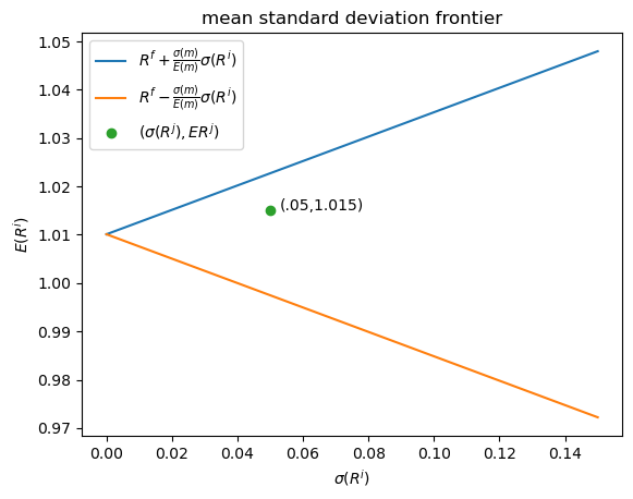
The figure shows two straight lines, the blue upper one being the locus of \(( \sigma(R^i), E(R^i)\) pairs that are on the mean-variance frontier or mean-standard-deviation frontier.
The green dot refers to a return \(R^j\) that is not on the frontier and that has moments \((\sigma(R^j), E R^j) = (.05, 1.015)\).
It is described by the statistical model
where \(R^i\) is a return that is on the frontier and \(\epsilon^j\) is a random variable that has mean zero and that is orthogonal to \(R^i\).
Then \( E R^j = E R^i\) and, as a consequence of \(R^j\) not being on the frontier,
The length of a horizontal line from the point \(\sigma(R^j), E (R^j) = .05, 1.015\) to the frontier equals
This is a measure of the part of the risk in \(R^j\) that is not priced because it is uncorrelated with the stochastic discount factor and so can be diversified away (i.e., averaged out to zero by holding a diversified portfolio).
41.7. Mathematical structure of frontier#
The mathematical structure of the mean-variance frontier described by inequality (41.6) implies that
all returns on the frontier are perfectly correlated.
Thus,
Let \(R^m, R^{mv}\) be two returns on the frontier.
Then for some scalar \(a\), a return \(R^{m v}\) on the mean-variance frontier satisfies the affine equation \(R^{m v}=R^{f}+a\left(R^{m}-R^{f}\right)\) . This is an exact equation with no residual.
each return \(R^{mv}\) that is on the mean-variance frontier is perfectly (negatively) correlated with \(m\)
\(\left(\rho_{m, R^{mv}}=-1\right) \Rightarrow \begin{cases} m=a+b R^{m v} \\ R^{m v}=e+d m \end{cases}\) for some scalars \(a, b, e, d\),
Therefore, any return on the mean-variance frontier is a legitimate stochastic discount factor
for any mean-variance-efficient return \(R^{m v}\) that is on the frontier but that is not \(R^{f}\), there exists a single-beta representation for any return \(R^i\) that takes the form:
the regression coefficient \(\beta_{i, R^{m v}}\) is often called asset \(i\)’s beta
The special case of a single-beta representation (41.7) with \( R^{i}=R^{m v}\) is
\(E R^{m v}=R^{f}+1 \cdot\left[E\left(R^{m v}\right)-R^{f}\right] \)
41.8. Multi-factor models#
The single-beta representation (41.7) is a special case of the multi-factor model
where \(\lambda_j\) is the price of being exposed to risk factor \(f_t^j\) and \(\beta_{i,j}\) is asset \(i\)’s exposure to that risk factor.
To uncover the \(\beta_{i,j}\)’s, one takes data on time series of the risk factors \(f_t^j\) that are being priced and specifies the following least squares regression
Special cases are:
a popular single-factor model specifies the single factor \(f_t\) to be the return on the market portfolio
another popular single-factor model called the consumption-based model specifies the factor to be \( m_{t+1} = \beta \frac{u^{\prime}\left(c_{t+1}\right)}{u^{\prime}\left(c_{t}\right)}\), where \(c_t\) is a representative consumer’s time \(t\) consumption.
As a reminder, model objects are interpreted as follows:
\(\beta_{i,a}\) is the exposure of return \(R^i\) to risk factor \(f_a\)
\(\lambda_{a}\) is the price of exposure to risk factor \(f_a\)
41.9. Empirical implementations#
We briefly describe empirical implementations of multi-factor generalizations of the single-factor model described above.
Two representations of a multi-factor model play importnt roles in empirical applications.
One is the time series regression (41.8)
The other representation entails a cross-section regression of average returns \(E R^i\) for assets \(i =1, 2, \ldots, I\) on prices of risk \(\lambda_j\) for \(j =a, b, c, \ldots\)
Here is the cross-section regression specification for a multi-factor model:
Testing strategies:
Time-series and cross-section regressions play roles in both estimating and testing beta representation models.
The basic idea is to implement the following two steps.
Step 1:
Estimate \(a_{i}, \beta_{i, a}, \beta_{i, b}, \cdots\) by running a time series regression: \(R_{t}^{i}\) on a constant and \(f_{t}^{a}, f_{t}^{b}, \ldots\)
Step 2:
take the \(\beta_{i, j}\)’s estimated in step one as regressors together with data on average returns \(E R^i\) over some period and then estimate the cross-section regression
Here \(\perp\) means orthogonal to
estimate \(\gamma, \lambda_{a}, \lambda_{b}, \ldots\) by an appropriate regression technique, recognizing that the regressors have been generated by a step 1 regression.
Note that presumably the risk-free return \(E R^{f}=\gamma\).
For excess returns \(R^{ei} = R^i - R^f\) we have
In the following exercises, we illustrate aspects of these empirical strategies on artificial data.
Our basic tools are random number generator that we shall use to create artificial samples that conform to the theory and least squares regressions that let us watch aspects of the theory at work.
These exercises will further convince us that asset pricing theory is mostly about covariances and least squares regressions.
41.10. Exercises#
Let’s start with some imports.
import numpy as np
import statsmodels.api as sm
import matplotlib.pyplot as plt
Lots of our calculations will involve computing population and sample OLS regressions.
So we define a function for simple univariate OLS regression that calls the OLS routine from statsmodels.
def simple_ols(X, Y, constant=False):

    if constant:
        X = sm.add_constant(X)

    model = sm.OLS(Y, X)
    res = model.fit()

    β_hat = res.params[-1]
    σ_hat = np.sqrt(res.resid @ res.resid / res.df_resid)

    return β_hat, σ_hat
Exercise 41.1
Look at the equation,
Verify that this equation is a regression equation.
Solution
To verify that it is a regression equation we must show that the residual is orthogonal to the regressor.
Our assumptions about mutual orthogonality imply that
It follows that
Exercise 41.2
Give a formula for the regression coefficient \(\beta_{i, R^m}\).
Solution
The regression coefficient \(\beta_{i, R^m}\) is
Exercise 41.3
As in many sciences, it is useful to distinguish a direct problem from an inverse problem.
A direct problem involves simulating a particular model with known parameter values.
An inverse problem involves using data to estimate or choose a particular parameter vector from a manifold of models indexed by a set of parameter vectors.
Please assume the parameter values provided below and then simulate 2000 observations from the theory specified above for 5 assets, \(i = 1, \ldots, 5\).
More Exercises
Now come some even more fun parts!
Our theory implies that there exist values of two scalars, \(a\) and \(b\), such that a legitimate stochastic discount factor is:
The parameters \(a, b\) must satisfy the following equations:
Solution
Direct Problem:
# Code for the direct problem

# assign the parameter values
ERf = 0.02
σf = 0.00 # Zejin: Hi tom, here is where you manipulate σf
ξ = 0.06
λ = 0.08
βi = np.array([0.2, .4, .6, .8, 1.0])
σi = np.array([0.04, 0.04, 0.04, 0.04, 0.04])
# in this cell we set the number of assets and number of observations
# we first set T to a large number to verify our computation results
T = 2000
N = 5
# simulate i.i.d. random shocks
e = np.random.normal(size=T)
u = np.random.normal(size=T)
ϵ = np.random.normal(size=(N, T))
# simulate the return on a risk-free asset
Rf = ERf + σf * e

# simulate the return on the market portfolio
excess_Rm = ξ + λ * u
Rm = Rf + excess_Rm

# simulate the return on asset i
Ri = np.empty((N, T))
for i in range(N):
    Ri[i, :] = Rf + βi[i] * excess_Rm + σi[i] * ϵ[i, :]
Now that we have a panel of data, we’d like to solve the inverse problem by assuming the theory specified above and estimating the coefficients given above.
# Code for the inverse problem
Inverse Problem:
We will solve the inverse problem by simple OLS regressions.
estimate \(E\left[R^f\right]\) and \(\sigma_f\)
ERf_hat, σf_hat = simple_ols(np.ones(T), Rf)
ERf_hat, σf_hat
(np.float64(0.020000000000000046), np.float64(4.5114090308141905e-17))
Let’s compare these with the true population parameter values.
ERf, σf
(0.02, 0.0)
\(\xi\) and \(\lambda\)
ξ_hat, λ_hat = simple_ols(np.ones(T), Rm - Rf)
ξ_hat, λ_hat
(np.float64(0.05767739282591654), np.float64(0.07864290083547071))
ξ, λ
(0.06, 0.08)
\(\beta_{i, R^m}\) and \(\sigma_i\)
βi_hat = np.empty(N)
σi_hat = np.empty(N)

for i in range(N):
    βi_hat[i], σi_hat[i] = simple_ols(Rm - Rf, Ri[i, :] - Rf)
βi_hat, σi_hat
(array([0.20364397, 0.40167354, 0.59144152, 0.80560113, 0.99168405]),
 array([0.0405601 , 0.03997942, 0.0404715 , 0.04122879, 0.0405056 ]))
βi, σi
(array([0.2, 0.4, 0.6, 0.8, 1. ]), array([0.04, 0.04, 0.04, 0.04, 0.04]))
Q: How close did your estimates come to the parameters we specified?
Exercise 41.4
Using the equations above, find a system of two linear equations that you can solve for \(a\) and \(b\) as functions of the parameters \((\lambda, \xi, E[R_f])\).
Write a function that can solve these equations.
Please check the condition number of a key matrix that must be inverted to determine a, b
Solution
The system of two linear equations is shown below:
# Code here
def solve_ab(ERf, σf, λ, ξ):

    M = np.empty((2, 2))
    M[0, 0] = ERf + ξ
    M[0, 1] = (ERf + ξ) ** 2 + λ ** 2 + σf ** 2
    M[1, 0] = ERf
    M[1, 1] = ERf ** 2 + ξ * ERf + σf ** 2

    a, b = np.linalg.solve(M, np.ones(2))
    condM = np.linalg.cond(M)

    return a, b, condM
Let’s try to solve \(a\) and \(b\) using the actual model parameters.
a, b, condM = solve_ab(ERf, σf, λ, ξ)
a, b, condM
(np.float64(87.49999999999999),
 np.float64(-468.7499999999999),
 np.float64(54.406619883717504))
Exercise 41.5
Using the estimates of the parameters that you generated above, compute the implied stochastic discount factor.
Solution
Now let’s pass \(\hat{E}(R^f), \hat{\sigma}^f, \hat{\lambda}, \hat{\xi}\) to the function solve_ab.
a_hat, b_hat, M_hat = solve_ab(ERf_hat, σf_hat, λ_hat, ξ_hat)
a_hat, b_hat, M_hat
(np.float64(86.22023105914293),
 np.float64(-466.29050926460025),
 np.float64(53.22127041011371))