25. Etymology of Entropy

This lecture describes and compares several notions of entropy.

Among the senses of entropy, we’ll encounter these

• A measure of uncertainty of a random variable advanced by Claude Shannon [SW49]

• A key object governing thermodynamics

• Kullback and Leibler’s measure of the statistical divergence between two probability distributions

• A measure of the volatility of stochastic discount factors that appear in asset pricing theory

• Measures of unpredictability that occur in classical Wiener-Kolmogorov linear prediction theory

• A frequency domain criterion for constructing robust decision rules

The concept of entropy plays an important role in robust control formulations described in this lecture Risk and Model Uncertainty and in this lecture Robustness.

25.1. Information Theory

In information theory [SW49], entropy is a measure of the unpredictability of a random variable.

To illustrate things, let \(X\) be a discrete random variable taking values \(x_1, \ldots, x_n\) with probabilities \(p_i = \textrm{Prob}(X = x_i) \geq 0, \sum_i p_i =1\).

Claude Shannon’s [SW49] definition of entropy is

(25.1)\[ H(p) = \sum_i p_i \log_b (p_i^{-1}) = - \sum_i p_i \log_b (p_i) . \]

where \(\log_b\) denotes the log function with base \(b\).

Inspired by the limit

\[ \lim_{p\downarrow 0} p \log p = \lim_{p \downarrow 0} \frac{\log p}{p^{-1}} = \lim_{p \downarrow 0}p = 0, \]

we set \(p \log p = 0\) in equation (25.1).

Typical bases for the logarithm are \(2\), \(e\), and \(10\).

In the information theory literature, logarithms of base \(2\), \(e\), and \(10\) are associated with units of information called bits, nats, and dits, respectively.

Shannon typically used base \(2\).

25.2. A Measure of Unpredictability

For a discrete random variable \(X\) with probability density \(p = \{p_i\}_{i=1}^n\), the surprisal for state \(i\) is \( s_i = \log\left(\frac{1}{p_i}\right) \).

The quantity \( \log\left(\frac{1}{p_i}\right) \) is called the surprisal because it is inversely related to the likelihood that state \(i\) will occur.

Note that entropy \(H(p)\) equals the expected surprisal

\[ H(p) = \sum_i p_i s_i = \sum_i p_i \log\left(\frac{1}{p_i} \right) = - \sum_i p_i \log\left(p_i \right). \]

25.2.1. Example

Take a possibly unfair coin, so \(X = \{0,1\}\) with \(p = {\rm Prob}(X=1) = p \in [0,1]\).

Then

\[ H(p) = -(1-p)\log (1-p) - p \log p. \]

Evidently,

\[ H'(p) = \log(1-p) - \log p = 0 \]

at \(p=.5\) and \(H''(p) = -\frac{1}{1-p} -\frac{1}{p} < 0\) for \(p\in (0,1)\).

So \(p=.5\) maximizes entropy, while entropy is minimized at \(p=0\) and \(p=1\).

Thus, among all coins, a fair coin is the most unpredictable.

See Fig. 25.1

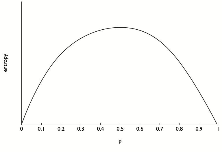
Fig. 25.1 Entropy as a function of \(\hat \pi_1\) when \(\pi_1 = .5\).

25.2.2. Example

Take an \(n\)-sided possibly unfair die with a probability distribution \(\{p_i\}_{i=1}^n\). The die is fair if \(p_i = \frac{1}{n} \forall i\).

Among all dies, a fair die maximizes entropy.

For a fair die, entropy equals \(H(p) = - n^{-1} \sum_i \log \left( \frac{1}{n} \right) = \log(n)\).

To specify the expected number of bits needed to isolate the outcome of one roll of a fair \(n\)-sided die requires \(\log_2 (n)\) bits of information.

For example, if \(n=2\), \(\log_2(2) =1\).

For \(n=3\), \(\log_2(3) = 1.585\).

25.3. Mathematical Properties of Entropy

For a discrete random variable with probability vector \(p\), entropy \(H(p)\) is a function that satisfies

• \(H\) is continuous.

• \(H\) is symmetric: \(H(p_1, p_2, \ldots, p_n) = H(p_{r_1}, \ldots, p_{r_n})\) for any permutation \(r_1, \ldots, r_n\) of \(1,\ldots, n\).

• A uniform distribution maximizes \(H(p)\): \( H(p_1, \ldots, p_n) \leq H(\frac{1}{n}, \ldots, \frac{1}{n}) .\)

• Maximum entropy increases with the number of states: \( H(\frac{1}{n}, \ldots, \frac{1}{n} ) \leq H(\frac{1}{n+1} , \ldots, \frac{1}{n+1})\).

• Entropy is not affected by events zero probability.

25.4. Conditional Entropy

Let \((X,Y)\) be a bivariate discrete random vector with outcomes \(x_1, \ldots, x_n\) and \(y_1, \ldots, y_m\), respectively, occurring with probability density \(p(x_i, y_i)\).

Conditional entropy \(H(X| Y)\) is defined as

(25.2)\[ H(X | Y) = \sum_{i,j} p(x_i,y_j) \log \frac{p(y_j)}{p(x_i,y_j)}. \]

Here \(\frac{p(y_j)}{p(x_i,y_j)}\), the reciprocal of the conditional probability of \(x_i\) given \(y_j\), can be defined as the conditional surprisal.

25.5. Independence as Maximum Conditional Entropy

Let \(m=n\) and \([x_1, \ldots, x_n ] = [y_1, \ldots, y_n]\).

Let \(\sum_j p(x_i,y_j) = \sum_j p(x_j, y_i) \) for all \(i\), so that the marginal distributions of \(x\) and \(y\) are identical.

Thus, \(x\) and \(y\) are identically distributed, but they are not necessarily independent.

Consider the following problem: choose a joint distribution \(p(x_i,y_j)\) to maximize conditional entropy (25.2) subject to the restriction that \(x\) and \(y\) are identically distributed.

The conditional-entropy-maximizing \(p(x_i,y_j)\) sets

\[ \frac{p(x_i,y_j)}{p(y_j)} = \sum_j p(x_i, y_j) = p(x_i) \forall i . \]

Thus, among all joint distributions with identical marginal distributions, the conditional entropy maximizing joint distribution makes \(x\) and \(y\) be independent.

25.6. Thermodynamics

Josiah Willard Gibbs (see https://en.wikipedia.org/wiki/Josiah_Willard_Gibbs) defined entropy as

(25.3)\[ S = - k_B \sum_i p_i \log p_i \]

where \(p_i\) is the probability of a micro state and \(k_B\) is Boltzmann’s constant.

• The Boltzmann constant \(k_b\) relates energy at the micro particle level with the temperature observed at the macro level. It equals what is called a gas constant divided by an Avogadro constant.

The second law of thermodynamics states that the entropy of a closed physical system increases until \(S\) defined in (25.3) attains a maximum.

25.7. Statistical Divergence

Let \(X\) be a discrete state space \(x_1, \ldots, x_n\) and let \(p\) and \(q\) be two discrete probability distributions on \(X\).

Assume that \(\frac{p_i}{q_t} \in (0,\infty)\) for all \(i\) for which \(p_i >0\).

Then the Kullback-Leibler statistical divergence, also called relative entropy, is defined as

(25.4)\[ D(p|q) = \sum_i p_i \log \left(\frac{p_i}{q_i}\right) = \sum_i q_i \left( \frac{p_i}{q_i}\right) \log\left( \frac{p_i}{q_i}\right) . \]

Evidently,

\[ \begin{aligned} D(p|q) & = - \sum_i p_i \log q_i + \sum_i p_i \log p_i \cr & = H(p,q) - H(p) , \end{aligned} \]

where \(H(p,q) = \sum_i p_i \log q_i\) is the cross-entropy.

It is easy to verify, as we have done above, that \( D(p|q) \geq 0\) and that \(D(p|q) = 0\) implies that \(p_i = q_i\) when \(q_i >0\).

25.8. Continuous distributions

For a continuous random variable, Kullback-Leibler divergence between two densities \(p\) and \(q\) is defined as

\[ D(p|q) = \int p(x) \log \left(\frac{p(x)}{q(x)} \right) d \, x . \]

25.9. Relative entropy and Gaussian distributions

We want to compute relative entropy for two continuous densities \(\phi\) and \(\hat \phi\) when \(\phi\) is \({\cal N}(0,I)\) and \({\hat \phi}\) is \({\cal N}(w, \Sigma)\), where the covariance matrix \(\Sigma\) is nonsingular.

We seek a formula for

\[ \textrm{ent} = \int (\log {\hat \phi(\varepsilon)} - \log \phi(\varepsilon) ){\hat \phi(\varepsilon)} d \varepsilon. \]

Claim

(25.5)\[ \textrm{ent} = %\int (\log {\hat \phi} - \log \phi ){\hat \phi} d \varepsilon= -{1 \over 2} \log \det \Sigma + {1 \over 2}w'w + {1 \over 2}\mathrm{trace} (\Sigma - I) . \]

Proof

The log likelihood ratio is

(25.6)\[ \log {\hat \phi}(\varepsilon) - \log \phi(\varepsilon) = {1 \over 2} \left[ - (\varepsilon - w)' \Sigma^{-1} (\varepsilon - w) + \varepsilon' \varepsilon - \log \det \Sigma\right] . \]

Observe that

\[ - \int {1 \over 2} (\varepsilon - w)' \Sigma^{-1} (\varepsilon - w) {\hat \phi}(\varepsilon) d\varepsilon = - {1 \over 2}\mathrm{trace}(I). \]

Applying the identity \(\varepsilon = w + (\varepsilon - w)\) gives

\[ {1\over 2}\varepsilon' \varepsilon = {1 \over 2}w' w + {1 \over 2} (\varepsilon - w)' (\varepsilon - w) + w' (\varepsilon - w). \]

Taking mathematical expectations

\[ {1 \over 2} \int \varepsilon' \varepsilon {\hat \phi}(\varepsilon) d \varepsilon = {1\over 2} w'w + {1 \over 2} \mathrm{trace}(\Sigma). \]

Combining terms gives

(25.7)\[ \textrm{ent} = \int (\log {\hat \phi} - \log \phi ){\hat \phi} d \varepsilon= -{1 \over 2} \log \det \Sigma + {1 \over 2}w'w + {1 \over 2}\mathrm{trace} (\Sigma - I) . \]

which agrees with equation (25.5). Notice the separate appearances of the mean distortion \(w\) and the covariance distortion \(\Sigma - I\) in equation (25.7).

Extension

Let \(N_0 = {\mathcal N}(\mu_0,\Sigma_0)\) and \(N_1={\mathcal N}(\mu_1, \Sigma_1)\) be two multivariate Gaussian distributions.

Then

(25.8)\[ D(N_0|N_1) = \frac{1}{2} \left(\mathrm {trace} (\Sigma_1^{-1} \Sigma_0) + (\mu_1 -\mu_0)' \Sigma_1^{-1} (\mu_1 - \mu_0) - \log\left( \frac{ \mathrm {det }\Sigma_0 }{\mathrm {det}\Sigma_1}\right) - k \right). \]

25.10. Von Neumann Entropy

Let \(P\) and \(Q\) be two positive-definite symmetric matrices.

A measure of the divergence between two \(P\) and \(Q\) is

\[ D(P|Q)= \textrm{trace} ( P \ln P - P \ln Q - P + Q) \]

where the log of a matrix is defined here (https://en.wikipedia.org/wiki/Logarithm_of_a_matrix).

A density matrix \(P\) from quantum mechanics is a positive definite matrix with trace \(1\).

The von Neumann entropy of a density matrix \(P\) is

\[ S = - \textrm{trace} (P \ln P) \]

25.11. Backus-Chernov-Zin Entropy

After flipping signs, [BCZ14] use Kullback-Leibler relative entropy as a measure of volatility of stochastic discount factors that they assert is useful for characterizing features of both the data and various theoretical models of stochastic discount factors.

Where \(p_{t+1}\) is the physical or true measure, \(p_{t+1}^*\) is the risk-neutral measure, and \(E_t\) denotes conditional expectation under the \(p_{t+1}\) measure, [BCZ14] define entropy as

(25.9)\[ L_t (p_{t+1}^*/p_{t+1}) = - E_t \log( p_{t+1}^*/p_{t+1}). \]

Evidently, by virtue of the minus sign in equation (25.9),

(25.10)\[ L_t (p_{t+1}^*/p_{t+1}) = D_{KL,t}( p_{t+1}^*|p_{t+1}), \]

where \(D_{KL,t}\) denotes conditional relative entropy.

Let \(m_{t+1}\) be a stochastic discount factor, \(r_{t+1}\) a gross one-period return on a risky security, and \((r_{t+1}^1)^{-1}\equiv q_t^1 = E_t m_{t+1}\) be the reciprocal of a risk-free one-period gross rate of return. Then

\[ E_t (m_{t+1} r_{t+1}) = 1 \]

[BCZ14] note that a stochastic discount factor satisfies

\[ m_{t+1} = q_t^1 p_{t+1}^*/p_{t+1} . \]

They derive the following entropy bound

\[ E L_t (m_{t+1}) \geq E (\log r_{t+1} - \log r_{t+1}^1 ) \]

which they propose as a complement to a Hansen-Jagannathan [HJ91] bound.

25.12. Wiener-Kolmogorov Prediction Error Formula as Entropy

Let \(\{x_t\}_{t=-\infty}^\infty\) be a covariance stationary stochastic process with mean zero and spectral density \(S_x(\omega)\).

The variance of \(x\) is

\[ \sigma_x^2 =\left( \frac{1}{2\pi}\right) \int_{-\pi}^\pi S_x (\omega) d \omega . \]

As described in chapter XIV of [Sar87], the Wiener-Kolmogorov formula for the one-period ahead prediction error is

(25.11)\[ \sigma_\epsilon^2 = \exp\left[\left( \frac{1}{2\pi}\right) \int_{-\pi}^\pi \log S_x (\omega) d \omega \right]. \]

Occasionally the logarithm of the one-step-ahead prediction error \(\sigma_\epsilon^2\) is called entropy because it measures unpredictability.

Consider the following problem reminiscent of one described earlier.

Problem:

Among all covariance stationary univariate processes with unconditional variance \(\sigma_x^2\), find a process with maximal one-step-ahead prediction error.

The maximizer is a process with spectral density

\[ S_x(\omega) = 2 \pi \sigma_x^2. \]

Thus, among all univariate covariance stationary processes with variance \(\sigma_x^2\), a process with a flat spectral density is the most uncertain, in the sense of one-step-ahead prediction error variance.

This no-patterns-across-time outcome for a temporally dependent process resembles the no-pattern-across-states outcome for the static entropy maximizing coin or die in the classic information theoretic analysis described above.

25.13. Multivariate Processes

Let \(y_t\) be an \(n \times 1\) covariance stationary stochastic process with mean \(0\) with matrix covariogram \(C_y(j) = E y_t y_{t-j}' \) and spectral density matrix

\[ S_y(\omega) = \sum_{j=-\infty}^\infty e^{- i \omega j} C_y(j), \quad \omega \in [-\pi, \pi]. \]

Let

\[ y_t = D(L) \epsilon_t \equiv \sum_{j=0}^\infty D_j \epsilon_t \]

be a Wold representation for \(y\), where \(D(0)\epsilon_t\) is a vector of one-step-ahead errors in predicting \(y_t\) conditional on the infinite history \(y^{t-1} = [y_{t-1}, y_{t-2}, \ldots ]\) and \(\epsilon_t\) is an \(n\times 1\) vector of serially uncorrelated random disturbances with mean zero and identity contemporaneous covariance matrix \(E \epsilon_t \epsilon_t' = I\).

Linear-least-squares predictors have one-step-ahead prediction error \(D(0) D(0)'\) that satisfies

(25.12)\[ \log \det [D(0) D(0)'] = \left(\frac{1}{2 \pi} \right) \int_{-\pi}^\pi \log \det [S_y(\omega)] d \omega. \]

Being a measure of the unpredictability of an \(n \times 1\) vector covariance stationary stochastic process, the left side of (25.12) is sometimes called entropy.

25.14. Frequency Domain Robust Control

Chapter 8 of [HS08b] adapts work in the control theory literature to define a frequency domain entropy criterion for robust control as

(25.13)\[ \int_\Gamma \log \det [ \theta I - G_F(\zeta)' G_F(\zeta) ] d \lambda(\zeta) , \]

where \(\theta \in (\underline \theta, +\infty)\) is a positive robustness parameter and \(G_F(\zeta)\) is a \(\zeta\)-transform of the objective function.

Hansen and Sargent [HS08b] show that criterion (25.13) can be represented as

(25.14)\[ \log \det [ D(0)' D(0)] = \int_\Gamma \log \det [ \theta I - G_F(\zeta)' G_F(\zeta) ] d \lambda(\zeta) , \]

for an appropriate covariance stationary stochastic process derived from \(\theta, G_F(\zeta)\).

This explains the moniker maximum entropy robust control for decision rules \(F\) designed to maximize criterion (25.13).

25.15. Relative Entropy for a Continuous Random Variable

Let \(x\) be a continuous random variable with density \(\phi(x)\), and let \(g(x) \) be a nonnegative random variable satisfying \(\int g(x) \phi(x) dx =1\).

The relative entropy of the distorted density \(\hat \phi(x) = g(x) \phi(x)\) is defined as

\[ \textrm{ent}(g) = \int g(x) \log g(x) \phi(x) d x . \]

Fig. 25.2 plots the functions \(g \log g\) and \(g -1\) over the interval \(g \geq 0\).

That relative entropy \(\textrm{ent}(g) \geq 0\) can be established by noting (a) that \(g \log g \geq g-1\) (see Fig. 25.2) and (b) that under \(\phi\), \(E g =1\).

Fig. 25.3 and Fig. 25.4 display aspects of relative entropy visually for a continuous random variable \(x\) for two densities with likelihood ratio \(g \geq 0\).

Where the numerator density is \({\mathcal N}(0,1)\), for two denominator Gaussian densities \({\mathcal N}(0,1.5)\) and \({\mathcal N}(0,.95)\), respectively, Fig. 25.3 and Fig. 25.4 display the functions \(g \log g\) and \(g -1\) as functions of \(x\).

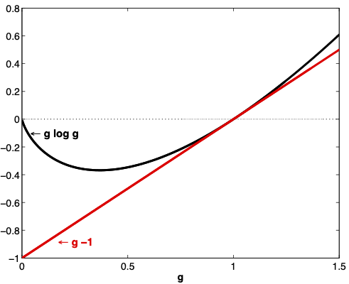
Fig. 25.2 The function \(g \log g\) for \(g \geq 0\). For a random variable \(g\) with \(E g =1\), \(E g \log g \geq 0\).

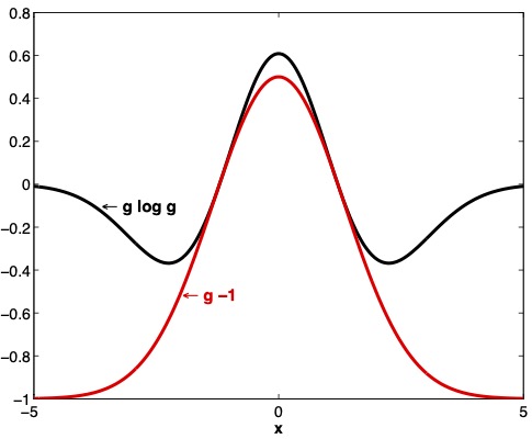
Fig. 25.3 Graphs of \(g \log g\) and \(g-1\) where \(g\) is the ratio of the density of a \({\mathcal N}(0,1)\) random variable to the density of a \({\mathcal N}(0,1.5)\) random variable. Under the \({\mathcal N}(0,1.5)\) density, \(E g =1\).

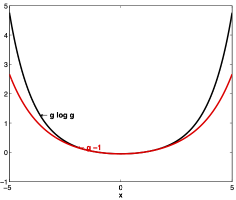
Fig. 25.4 \(g \log g\) and \(g-1\) where \(g\) is the ratio of the density of a \({\mathcal N}(0,1)\) random variable to the density of a \({\mathcal N}(0,1.5)\) random variable. Under the \({\mathcal N}(0,1.5)\) density, \(E g =1\).