20. Permanent Income Model using the DLE Class #

Contents

Permanent Income Model using the DLE Class
- The Permanent Income Model

This lecture is part of a suite of lectures that use the quantecon DLE class to instantiate models within the [HS13] class of models described in detail in Recursive Models of Dynamic Linear Economies.

In addition to what’s included in Anaconda, this lecture uses the quantecon library.

!pip install --upgrade quantecon

This lecture adds a third solution method for the linear-quadratic-Gaussian permanent income model with \(\beta R = 1\), complementing the other two solution methods described in Optimal Savings I: The Permanent Income Model and Optimal Savings II: LQ Techniques and this Jupyter notebook.

The additional solution method uses the DLE class.

In this way, we map the permanent income model into the framework of Hansen & Sargent (2013) “Recursive Models of Dynamic Linear Economies” [HS13].

We’ll also require the following imports

import numpy as np
import matplotlib.pyplot as plt
%matplotlib inline
from quantecon import DLE

np.set_printoptions(suppress=True, precision=4)

20.1. The Permanent Income Model #

The LQ permanent income model is an example of a savings problem.

A consumer has preferences over consumption streams that are ordered by the utility functional

(20.1)#\[E_0 \sum_{t=0}^\infty \beta^t u(c_t)\]

where \(E_t\) is the mathematical expectation conditioned on the consumer’s time \(t\) information, \(c_t\) is time \(t\) consumption, \(u(c)\) is a strictly concave one-period utility function, and \(\beta \in (0,1)\) is a discount factor.

The LQ model gets its name partly from assuming that the utility function \(u\) is quadratic:

\[ u(c) = -.5(c - \gamma)^2 \]

where \(\gamma>0\) is a bliss level of consumption.

The consumer maximizes the utility functional (20.1) by choosing a consumption, borrowing plan \(\{c_t, b_{t+1}\}_{t=0}^\infty\) subject to the sequence of budget constraints

(20.2)#\[c_t + b_t = R^{-1} b_{t+1} + y_t, t \geq 0\]

where \(y_t\) is an exogenous stationary endowment process, \(R\) is a constant gross risk-free interest rate, \(b_t\) is one-period risk-free debt maturing at \(t\), and \(b_0\) is a given initial condition.

We shall assume that \(R^{-1} = \beta\).

Equation (20.2) is linear.

We use another set of linear equations to model the endowment process.

In particular, we assume that the endowment process has the state-space representation

(20.3)#\[\begin{aligned} z_{t+1} & = A_{22} z_t + C_2 w_{t+1} \cr y_t & = U_y z_t \cr \end{aligned}\]

where \(w_{t+1}\) is an IID process with mean zero and identity contemporaneous covariance matrix, \(A_{22}\) is a stable matrix, its eigenvalues being strictly below unity in modulus, and \(U_y\) is a selection vector that identifies \(y\) with a particular linear combination of the \(z_t\).

We impose the following condition on the consumption, borrowing plan:

(20.4)#\[E_0 \sum_{t=0}^\infty \beta^t b_t^2 < +\infty\]

This condition suffices to rule out Ponzi schemes.

(We impose this condition to rule out a borrow-more-and-more plan that would allow the household to enjoy bliss consumption forever)

The state vector confronting the household at \(t\) is

\[\begin{split} x_t = \begin{bmatrix} z_t \\ b_t \end{bmatrix} \end{split}\]

where \(b_t\) is its one-period debt falling due at the beginning of period \(t\) and \(z_t\) contains all variables useful for forecasting its future endowment.

We assume that \(\{y_t\}\) follows a second order univariate autoregressive process:

\[ y_{t+1} = \alpha + \rho_1 y_t + \rho_2 y_{t-1} + \sigma w_{t+1} \]

20.1.1. Solution with the DLE Class#

One way of solving this model is to map the problem into the framework outlined in Section 4.8 of [HS13] by setting up our technology, information and preference matrices as follows:

Technology: \(\phi_c= \left[ {\begin{array}{c} 1 \\ 0 \end{array} } \right]\) , \(\phi_g= \left[ {\begin{array}{c} 0 \\ 1 \end{array} } \right]\) , \(\phi_i= \left[ {\begin{array}{c} -1 \\ -0.00001 \end{array} } \right]\), \(\Gamma= \left[ {\begin{array}{c} -1 \\ 0 \end{array} } \right]\), \(\Delta_k = 0\), \(\Theta_k = R\).

Information: \(A_{22} = \left[ {\begin{array}{ccc} 1 & 0 & 0 \\ \alpha & \rho_1 & \rho_2 \\ 0 & 1 & 0 \end{array} } \right]\), \(C_{2} = \left[ {\begin{array}{c} 0 \\ \sigma \\ 0 \end{array} } \right]\), \(U_b = \left[ {\begin{array}{ccc} \gamma & 0 & 0 \end{array} } \right]\), \(U_d = \left[ {\begin{array}{ccc} 0 & 1 & 0 \\ 0 & 0 & 0 \end{array} } \right]\).

Preferences: \(\Lambda = 0\), \(\Pi = 1\), \(\Delta_h = 0\), \(\Theta_h = 0\).

We set parameters

\(\alpha = 10, \beta = 0.95, \rho_1 = 0.9, \rho_2 = 0, \sigma = 1\)

(The value of \(\gamma\) does not affect the optimal decision rule)

The chosen matrices mean that the household’s technology is:

\[ c_t + k_{t-1} = i_t + y_t \]

\[ \frac{k_t}{R} = i_t \]

\[ l_t^2 = (0.00001)^2i_t \]

Combining the first two of these gives the budget constraint of the permanent income model, where \(k_t = b_{t+1}\).

The third equation is a very small penalty on debt-accumulation to rule out Ponzi schemes.

We set up this instance of the DLE class below:

α, β, ρ_1, ρ_2, σ = 10, 0.95, 0.9, 0, 1

γ = np.array([[-1], [0]])
ϕ_c = np.array([[1], [0]])
ϕ_g = np.array([[0], [1]])
ϕ_1 = 1e-5
ϕ_i = np.array([[-1], [-ϕ_1]])
δ_k = np.array([[0]])
θ_k = np.array([[1 / β]])
β = np.array([[β]])
l_λ = np.array([[0]])
π_h = np.array([[1]])
δ_h = np.array([[0]])
θ_h = np.array([[0]])

a22 = np.array([[1,   0,   0],
                [α, ρ_1, ρ_2],
                [0, 1, 0]])

c2 = np.array([[0], [σ], [0]])
ud = np.array([[0, 1, 0],
               [0, 0, 0]])
ub = np.array([[100, 0, 0]])

x0 = np.array([[0], [0], [1], [0], [0]])

info1 = (a22, c2, ub, ud)
tech1 = (ϕ_c, ϕ_g, ϕ_i, γ, δ_k, θ_k)
pref1 = (β, l_λ, π_h, δ_h, θ_h)
econ1 = DLE(info1, tech1, pref1)

To check the solution of this model with that from the LQ problem, we select the \(S_c\) matrix from the DLE class.

The solution to the DLE economy has:

\[ c_t = S_c x_t \]

econ1.Sc

array([[ 0.    , -0.05  , 65.5172,  0.3448,  0.    ]])

The state vector in the DLE class is:

\[\begin{split} x_t = \left[ {\begin{array}{c} h_{t-1} \\ k_{t-1} \\ z_t \end{array} } \right] \end{split}\]

where \(k_{t-1}\) = \(b_{t}\) is set up to be \(b_t\) in the permanent income model.

The state vector in the LQ problem is \(\begin{bmatrix} z_t \\ b_t \end{bmatrix}\).

Consequently, the relevant elements of econ1.Sc are the same as in \(-F\) occur when we apply other approaches to the same model in the lecture Optimal Savings II: LQ Techniques and this Jupyter notebook.

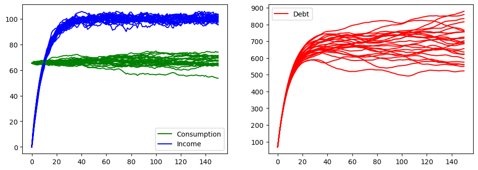
The plot below quickly replicates the first two figures of that lecture and that notebook to confirm that the solutions are the same

fig, (ax1, ax2) = plt.subplots(1, 2, figsize=(12, 4))

for i in range(25):
    econ1.compute_sequence(x0, ts_length=150)
    ax1.plot(econ1.c[0], c='g')
    ax1.plot(econ1.d[0], c='b')
ax1.plot(econ1.c[0], label='Consumption', c='g')
ax1.plot(econ1.d[0], label='Income', c='b')
ax1.legend()

for i in range(25):
    econ1.compute_sequence(x0, ts_length=150)
    ax2.plot(econ1.k[0], color='r')
ax2.plot(econ1.k[0], label='Debt', c='r')
ax2.legend()
plt.show()

_images/f8e3635c1496bcf1ee5787a8538ad2eb1d6d759d58bdf6a901071a5346826ccd.png

20. Permanent Income Model using the DLE Class#

20.1. The Permanent Income Model#

20.1.1. Solution with the DLE Class#

20. Permanent Income Model using the DLE Class #

20.1. The Permanent Income Model #