16. Composite Sorting#
16.1. Overview#
Optimal transport theory studies how a marginal probability measure can be related to another marginal probability measure in an ideal way.
here ideal means to minimize some cost criterion.
The output of such a theory is a coupling of the two probability measures, i.e., a joint probability measure having those two marginal probability measures.
This lecture describes how Job Boerma, Aleh Tsyvinski, Ruodu Wang, and Zhenyuan Zhang [Boerma et al., 2024] used optimal transport theory to formulate and compute an equilibrium of a model in which wages and allocations of workers across jobs adjust to match measures of different types with measures of different types of occupations.
Production technologies allow firms to reshape costs of mismatch so that they become concave.
It is then possible that in equilibrium there is neither positive assortative nor negative assortative matching, an outcome that [Boerma et al., 2024] call composite assortative matching.
For example, with composite matching in an equilibrium model with workers of different types, ex ante identical workers can sort into different occupations, some positively and some negatively.
[Boerma et al., 2024] show how composite matching can generate distinct non-trivial frequency distributions of labor earnings within and across occupations.
This lecture describes the [Boerma et al., 2024] model and presents Python code for computing equilibria.
The lecture then applies the code to the [Boerma et al., 2024] model of labor markets.
As with an earlier QuantEcon lecture on optimal transport, a key tool will be linear programming.
As we’ll see, [Boerma et al., 2024] also deploy dynamic programming in creative ways at important points in their analysis. So as you read this lecture, please watch for Bellman equations that might remind you of ideas encountered in this earlier QuantEcon lecture and this QuantEcon book.
16.2. Setup#
\(X\) and \(Y\) are finite sets that represent two distinct types of people to be matched.
For each \(x \in X,\) let a positive integer \(n_x\) be the number of agents of type \(x\).
Similarly, let a positive integer \(m_y\) be the agents of agents of type \(y \in Y\).
We refer to these two measures as marginals.
We assume that
so that the matching problem is balanced.
Given a cost function \(c \colon X \times Y \rightarrow \mathbb{R}\), the (discrete) optimal transport problem is
Given our discreteness assumptions about \(X\) and \(Y\), the problem admits an integer solution \(\mu \in \mathbb{Z}_+^{X \times Y}\), i.e., \(\mu_{xy}\) is a non-negative integer for each \(x\in X, y\in Y\).
We will study integer solutions.
Two points about restricting ourselves to integer solutions are worth mentioning:
it is without loss of generality for computational purposes, since every problem with float marginals can be transformed into an equivalent problem with integer marginals;
although the mathematical structure that we present actually works for arbitrary real marginals, some of our Python implementations would fail to work with float arithmetic.
We focus on a specific instance of an optimal transport problem:
We assume that \(X\) and \(Y\) are finite subsets of \(\mathbb{R}\) and that the cost function satisfies \(c_{xy} = h(|x - y|)\) for all \(x,y \in \mathbb{R},\) for an \(h: \mathbb{R}_+ \rightarrow \mathbb{R}_+\) that is strictly concave and strictly increasing and grounded (i.e., \(h(0)=0\)).
Such an \(h\) satisfies the following
Lemma. If \(h \colon \mathbb{R}_+ \rightarrow \mathbb{R}_+\) is strictly concave and grounded, then \(h\) is strictly subadditive, i.e. for all \(x,y\in \mathbb{R}_+, 0< x < y,\) we have
Proof. For \(\alpha \in (0,1)\) and \(x >0\) we have, by strict concavity and groundedness, \(h(\alpha x) > \alpha h(x) + (1-\alpha) h(0)=\alpha h(x)\).
Now fix \(x,y\in \mathbb{R}_+, 0< x < y,\) and let \(\alpha = \frac{x}{x+y};\) the previous observation gives \(h(x) = h(\alpha (x+y)) > \alpha h(x+y)\) and \(h(y) = h((1-\alpha) (x+y)) > (1-\alpha) h(x+y) \); summing these inequality delivers the result. \(\square\)
In the following implementation we assume that the cost function is \(c_{xy} = |x-y|^{1/\zeta}\) for \(\zeta>1,\) i.e. \(h(z) = z^{1/\zeta}\) for \(z \in \mathbb{R}_+.\)
Hence, our problem is
Let’s start setting up some Python code.
We use the following imports:
import numpy as np
from scipy.optimize import linprog
from itertools import chain
import pandas as pd
from collections import namedtuple


import matplotlib.pyplot as plt
import matplotlib.patches as patches
from matplotlib.ticker import MaxNLocator
from matplotlib import cm
from matplotlib.colors import Normalize
The following Python class takes as inputs sets of types \(X,Y \subset \mathbb{R},\) marginals \(n, m \) with positive integer entries such that \(\sum_{x \in X} n_x = \sum_{y \in Y} m_y \) and cost parameter \(\zeta>1\).
The cost function is stored as an \(|X| \times |Y|\) matrix with \((x,y)\)-entry equal to \(|x-y|^{1/\zeta},\) i.e., the cost of matching an agent of type \(x \in X\) with an agent of type \(y \in Y.\)
class ConcaveCostOT():
    def __init__(self, X_types=None, Y_types=None, n_x =None, m_y=None, ζ=2):

        # Sets of types
        self.X_types, self.Y_types = X_types, Y_types

        # Marginals
        if X_types is not None and Y_types is not None:
            non_empty_types = True
            self.n_x = np.ones(len(X_types), dtype=int) if n_x is None else n_x
            self.m_y = np.ones(len(Y_types), dtype=int) if m_y is None else m_y
        else:
            non_empty_types = False
            self.n_x, self.m_y = n_x, m_y

        # Cost function: |X|x|Y| matrix
        self.ζ = ζ
        if non_empty_types:
            self.cost_x_y = np.abs(X_types[:, None] - Y_types[None, :]) \
            ** (1 / ζ)
        else:
            self.cost_x_y = None
Let’s consider a random instance with given numbers of types \(|X|\) and \(|Y|\) and a given number of agents.
First, we generate random types \(X\) and \(Y.\)
Then we generate random quantities for each type so that there are \(N\) agents for each side.
number_of_x_types = 20
number_of_y_types = 20
N_agents_per_side = 60

np.random.seed(1)

## Generate random types
# generate random support for distributions of types
support_size = 50
random_support = np.unique(np.random.uniform(0,200, size=support_size))

# generate types
X_types_example = np.random.choice(random_support,
                    size=number_of_x_types, replace=False)
Y_types_example = np.random.choice(random_support,
                    size=number_of_y_types, replace=False)

## Generate random integer types quantities summing to N_agents_per_side

# generate integer vectors of lenght n_types summing to n_agents
def random_marginal(n_types, n_agents):
    cuts = np.sort(np.random.choice(np.arange(1,n_agents),
                                    size= n_types-1, replace=False))
    segments = np.diff(np.concatenate(([0], cuts, [n_agents])))
    return segments

# Create a method to assign random marginals to our class
def assign_random_marginals(self,random_seed):
    np.random.seed(random_seed)
    self.n_x = random_marginal(len(self.X_types), N_agents_per_side)
    self.m_y = random_marginal(len(self.Y_types), N_agents_per_side)

ConcaveCostOT.assign_random_marginals = assign_random_marginals

# Create an instance of our class and generate random marginals
example_pb = ConcaveCostOT(X_types_example, Y_types_example, ζ=2)
example_pb.assign_random_marginals(random_seed=1)
We use \(F\) (resp. \(G\)) to denote the cumulative distribution function associated to the measure \(n\) (resp. \(m\))
Thus, \(F(z) =\sum_{x \leq z: n_x > 0} n_x \) and \(G(z) =\sum_{y \leq z: m_y > 0} m_y \) for \(z\in \mathbb{R}.\)
Notice that we not normalizing the measures so \(F(\infty) = G(\infty) =N.\)
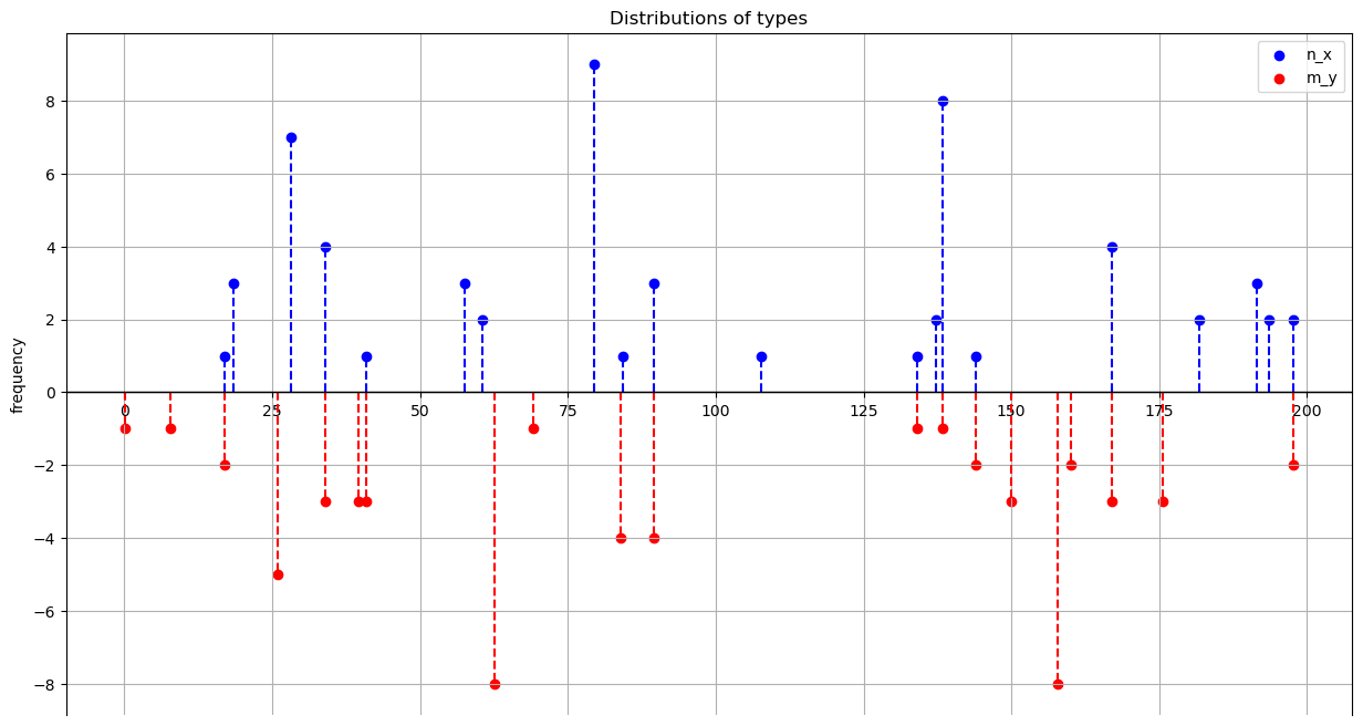
The following method plots the marginals on the real line
blue for \(X\) types,
red for \(Y\) types.
Note that there are possible overlaps between \(X\) and \(Y.\)
def plot_marginals(self, figsize=(15, 8), title='Distributions of types'):

    plt.figure(figsize=figsize)

    # Scatter plot n_x
    plt.scatter(self.X_types, self.n_x, color='blue', label='n_x')
    plt.vlines(self.X_types, ymin=0, ymax= self.n_x,
               color='blue', linestyles='dashed')

    # Scatter plot m_y
    plt.scatter(self.Y_types, - self.m_y, color='red', label='m_y')
    plt.vlines(self.Y_types, ymin=0, ymax=- self.m_y,
               color='red', linestyles='dashed')

    # Add grid and y=0 axis
    plt.grid(True)
    plt.axhline(0, color='black', linewidth=1)
    plt.gca().spines['bottom'].set_position(('data', 0))

    # Labeling the axes and the title
    plt.ylabel('frequency')
    plt.title(title)
    plt.gca().yaxis.set_major_locator(MaxNLocator(integer=True))
    plt.legend()
    plt.show()

ConcaveCostOT.plot_marginals = plot_marginals
example_pb.plot_marginals()
16.3. Characterization of primal solution#
16.3.1. Three properties of an optimal solution#
We now indicate important properties that are satisfied by an optimal solution.
Maximal number of perfect pairs
No intersecting pairs
Layering
Maximal number of perfect pairs
If \((z,z) \in X \times Y\) for some \(z \in \mathbb{R}\) then in each optimal solution there are \(\min\{n_z,m_z\}\) matches between type \(z \in X\) and \(z \in Y\).
Indeed, assume by contradiction that at an optimal solution we have \((z,y)\) and \((x,z)\) matched in positive amounts for \(y,x \neq z\).
We can verify that reassigning the minimum of such quantities to the pairs \((z,z)\) and \((x,y)\) improves upon the current matching since
where the first inequality follows from triangle inequality and the fact that \(h\) is increasing and the strict inequality from strict subadditivity.
We can then repeat the operation for any other analogous pair of matches involving \(z,\) while improving the value, until we have mass \(\min\{n_z,m_z\}\) on match \((z,z).\)
Viewing the matching \(\mu\) as a measure on \(X \times Y\) with marginals \(n\) and \(m\), this property says that in any optimal \(\mu\) we have \(\mu_{zz} = n_z \wedge m_z\) for \((z,z)\) in the diagonal \(\{(x,y) \in X \times Y: x=y\}\) of \(\mathbb{R} \times \mathbb{R}\).
The following method finds perfect pairs and returns the on-diagonal matchings as well as the residual off-diagonal marginals.
def match_perfect_pairs(self):

    # Find pairs on diagonal and related mass
    perfect_pairs_x, perfect_pairs_y = np.where(
                        self.X_types[:,None] == self.Y_types[None,:])
    Δ_q = np.minimum(self.n_x[perfect_pairs_x] ,self.m_y[perfect_pairs_y])

    # Compute off-diagonal residual masses for each side
    n_x_off_diag = self.n_x.copy()
    n_x_off_diag[perfect_pairs_x]-= Δ_q

    m_y_off_diag = self.m_y.copy()
    m_y_off_diag[perfect_pairs_y] -= Δ_q

    # Compute on-diagonal matching
    matching_diag = np.zeros((len(self.X_types), len(self.Y_types)), dtype=int)
    matching_diag[perfect_pairs_x, perfect_pairs_y] = Δ_q

    return n_x_off_diag, m_y_off_diag , matching_diag

ConcaveCostOT.match_perfect_pairs = match_perfect_pairs
n_x_off_diag, m_y_off_diag , matching_diag = example_pb.match_perfect_pairs()
print(f"On-diagonal matches: {matching_diag.sum()}")
print(f"Residual types in X: {len(n_x_off_diag[n_x_off_diag >0])}")
print(f"Residual types in Y: {len(m_y_off_diag[m_y_off_diag >0])}")
On-diagonal matches: 15
Residual types in X: 14
Residual types in Y: 16
We can therefore create a new instance with the residual marginals that will feature no perfect pairs.
Later we shall add the on-diagonal matching to the solution of this new instance.
We refer to this instance as “off-diagonal” since the product measure of the residual marginals \(n \otimes m\) feature zeros mass on the diagonal of \(\mathbb{R} \times \mathbb{R}.\)
In the rest of this section, we will focus on this instance.
We create a subclass to study the residual off-diagonal problem.
The subclass inherits the attributes and the modules from the original class.
We let \(Z := X \sqcup Y ,\) where \(\sqcup\) denotes the union of disjoint sets. We will
index types \(X\) as \(\{0, \dots,|X|-1\}\) and types \(Y\) as \(\{|X|, \dots,|X| + |Y|-1\};\)
store the cost function as a \(|Z| \times |Z|\) matrix with entry \((z,z')\) equal to \(c_{xy}\) if \(z=x \in X\) and \(z' =y\in Y\) or \(z=y \in Y\) and \(z' =x\in X\) or equal to \(+\infty\) if \(z\) and \(z'\) belong to the same side
(the latter is just customary, since these “infinitely penalized” entries are actually never accessed in the implementation);
let \(q\) be a vector of size \(|Z|\) whose \(z\)-th entry equals \(n_x\) if type \(x\) is the \(z\)-th smallest type in \(Z\) and \(-m_y\) if type \(y\) is the \(z\)-th smallest type in \(Z\); hence \(q\) encodes capacities of both sides on the (ascending) sorted set of types.
Finally, we add a method to flexibly add a pair \((i,j)\) with \(i \in \{0, \dots,|X|-1\},j \in \{|X|, \dots,|X| + |Y|-1\}\) or \(j \in \{0, \dots,|X|-1\},i \in \{|X|, \dots,|X| + |Y|-1\}\) to a matching matrix of size \(|X| \times |Y|\).
class OffDiagonal(ConcaveCostOT):
    def __init__(self, X_types, Y_types, n_x, m_y, ζ):
        super().__init__(X_types, Y_types, n_x, m_y, ζ)

        # Types (unsorted)
        self.types_list = np.concatenate((X_types,Y_types))

        # Cost function: |Z|x|Z| matrix
        self.cost_z_z = np.ones((len(self.types_list),
                                 len(self.types_list))) * np.inf

        # upper-right block
        self.cost_z_z[:len(self.X_types), len(self.X_types):] = self.cost_x_y

        # lower-left block
        self.cost_z_z[len(self.X_types):, :len(self.X_types)] = self.cost_x_y.T

        ## Distributions of types
        # sorted types and index identifier for each z in support
        self.type_z = np.argsort(self.types_list)
        self.support_z = self.types_list[self.type_z]

        # signed quantity for each type z
        self.q_z = np.concatenate([n_x, - m_y])[self.type_z]

    # Mathod that adds to matching matrix a pair (i,j)
    def add_pair_to_matching(self, pair_ids, matching):
        if pair_ids[0] < pair_ids[1]:
            # the pair of indices correspond to a pair (x,y)
            matching[pair_ids[0], pair_ids[1]-len(self.X_types)] = 1
        else:
            # the pair of indices correspond to a pair (y,x)
            matching[pair_ids[1], pair_ids[0]-len(self.X_types)] = 1
We add a function that returns an instance of the off-diagonal subclass as well as the on-diagonal matching and the indices of the residual off-diagonal types.
These indices will come handy for adding the off-diagonal matching matrix to the diagonal matching matrix we just found, since the former will have a smaller size if there are perfect pairs in the original problem.
def generate_offD_onD_matching(self):
    # Match perfect pairs and compute on-diagonal matching
    n_x_off_diag, m_y_off_diag , matching_diag = self.match_perfect_pairs()

    # Find indices of residual non-zero quantities for each side
    nonzero_id_x = np.flatnonzero(n_x_off_diag)
    nonzero_id_y = np.flatnonzero(m_y_off_diag)

    # Create new instance with off-diagonal types
    off_diagonal = OffDiagonal(self.X_types[nonzero_id_x],
                                    self.Y_types[nonzero_id_y],
                                    n_x_off_diag[nonzero_id_x],
                                    m_y_off_diag[nonzero_id_y],
                                    self.ζ)

    return off_diagonal, (nonzero_id_x, nonzero_id_y, matching_diag)

ConcaveCostOT.generate_offD_onD_matching = generate_offD_onD_matching
We apply it to our example:
example_off_diag, _ = example_pb.generate_offD_onD_matching()
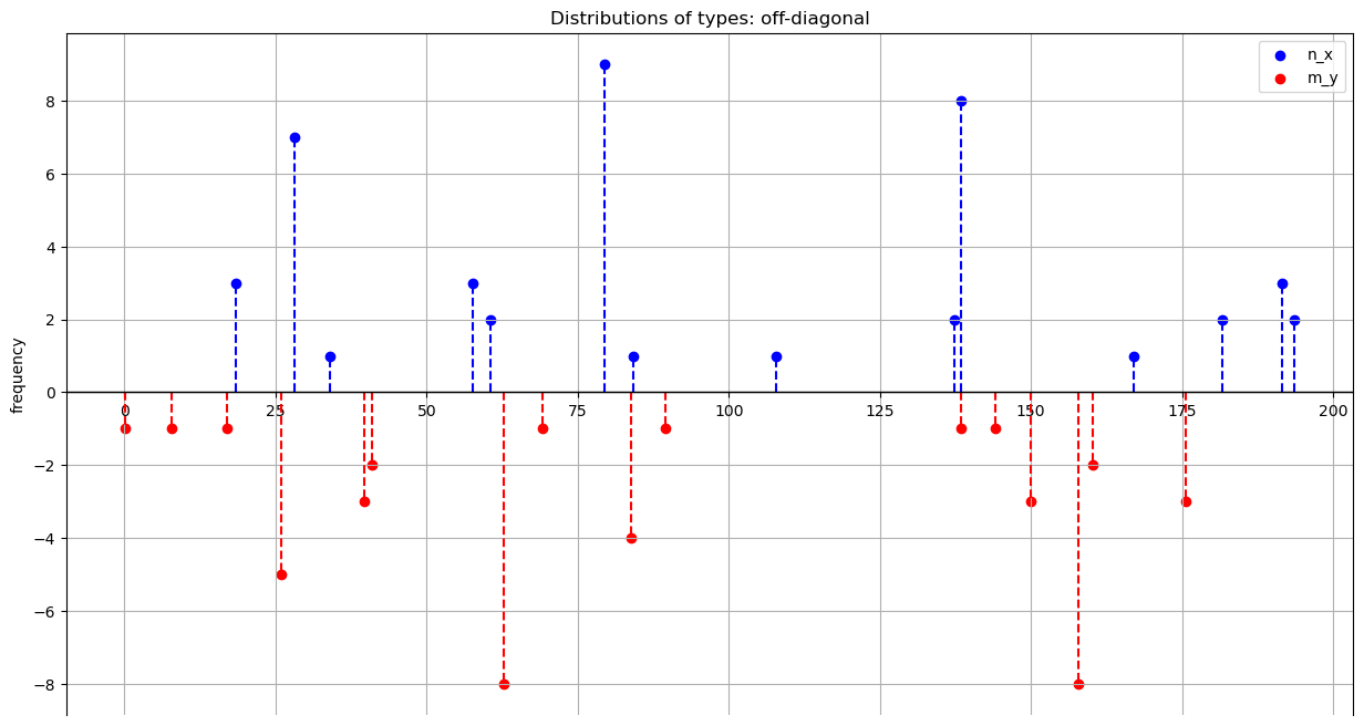
Let’s plot the residual marginals to verify visually that there are no overlappings between types from distinct sides in the off-diagonal instance.
example_off_diag.plot_marginals(title='Distributions of types: off-diagonal')
To prepare the way for the second property, represent both types on the real line and draw semicirles that join \((x,y)\) for all pairs \((x,y) \in X \times Y\) that are matched in a solution.
In terms of these semicircles we assert the
No intersecting pairs property
unless they share one of the endpoints, the semicirles do not intersect.
To prove the property, we reason by contradiction.
Let’s consider types \(x,x' \in X\) and \(y,y' \in Y.\)
Matched pairs cain “intersect” (or be tangent).
We will show that in both cases the partial matching among types \(x,x',y,y'\) can be improved by uncrossing, i.e. reassigning the quantities while improving on the solution and reducing the number of intersecting pairs.
The first case of intersecting pairs is
with pairs \((x,y')\) and \((x',y)\) matched in positive quantities.
Then it follows from strict monotonicity of \(h\) that \(h(|x-y|) < h(|x-y'|)\) and \(h(|x'-y'|) < h(|x'-y|),\) hence \(h(|x-y|)+ h(|x'-y'|) < h(|x-y'|) + h(|x'-y|).\)
Therefore, we can take the minimum of the masses of the matched pairs \((x,y')\) and \((x',y)\) and reallocate it to the pairs \((x,y)\) and \((x',y')\), therby strictly improving the cost among \(x,y,x',y'.\)
The second case of intersecting pairs is
with pairs \((x,y')\) and \((x',y)\) matched.
In this case we have
Letting \( \alpha := \frac{|x-y'| - |x'-y'|}{|x-y| - |x'-y'|} \in (0,1), \) we have
Hence, by strict concavity of \( h, \)
Adding the two inequalities:
Therefore, as in the first case, we can strictly improve the cost among \(x,y,x',y'\) by uncrossing the pairs.
Finally, it remains to argue that in both cases uncrossing operations do not increase the number of intersections with other matched pairs.
It can indeed be shown on a case-by-case basis that, in both of the above cases, for any other matched pair \((x'',y'')\) the number of intersections between pairs \((x,y), (x',y')\) and the pair \((x'',y'')\) (i.e., after uncrossing) is not larger than the number of intersections between pairs \((x,y'), (x',y)\) and the pair \((x'',y'')\) (i.e., before uncrossing), hence the uncrossing operations above reduce the number of intersections.
We conclude that if a matching features intersecting pairs, it can be modified via a sequence of uncrossing operations into a matching without intersecting pairs while improving on the value.
We now consider the third property.
Layering
Recall that there are \(2N\) individual agents, each agent \(i\) having type \(z_i \in X \sqcup Y.\)
When we introduce the off diagonal matching, to stress that the types sets are disjoint now.
To simplify our explanation of this property, assume for now that each agent has its own distinct type (i.e., \(|X| = |Y| =N\) and \(n=m= \mathbf{1}_N\)), in which case the optimal transport problem is also referred to as assignment problem.
Let’s index agents according to their types:
Suppose that agents \(i\) of type \(z_i\) and \(j\) of type \(z_j\), with \(z_i < z_j,\) are matched in a particular optimal solution.
Then there is an equal number of agents from each side in \(\{i+1, \dots, j-1\},\) if this set is not empty.
Indeed, if this were not the case, then some agent \(k \in \{i+1,j-1\}\) would be matched with some agent \(\ell\) with \(\ell \notin \{i,\dots, j\},\) i.e., there would be types
with matches \((z_i,z_j)\) and \((z_k, z_\ell),\) violating the no intersecting pairs property.
We conclude that we can define a binary relation on \([N]\) such that \(i \sim j\) if there is an equal number of agents of each side in \(\{i,i+1,\dots, j\}\) (or if this set is empty).
This is an equivalence relation, so we can find associated equivalence classes that we call layers.
By the reasoning above, in an optimal solution all pairs \(i,j\) (of opposite sides) which are matched belong to the same layer, hence we can solve the assignment problem associated to each layer and then add up the solutions.
In terms of distributions, \(i\) and \(j,\) of types \(x \in X\) and \(y \in Y\) respectively, belong to the same layer (i.e., \(x \sim y\)) if and only if \(F(y-) - F(x) = G(y-) - G(x).\)
If \(F\) and \(G\) were continuous, then \(F(y) - F(x) = G(y) - G(x) \iff F(x) - G(x) = F(y) - G(y).\)
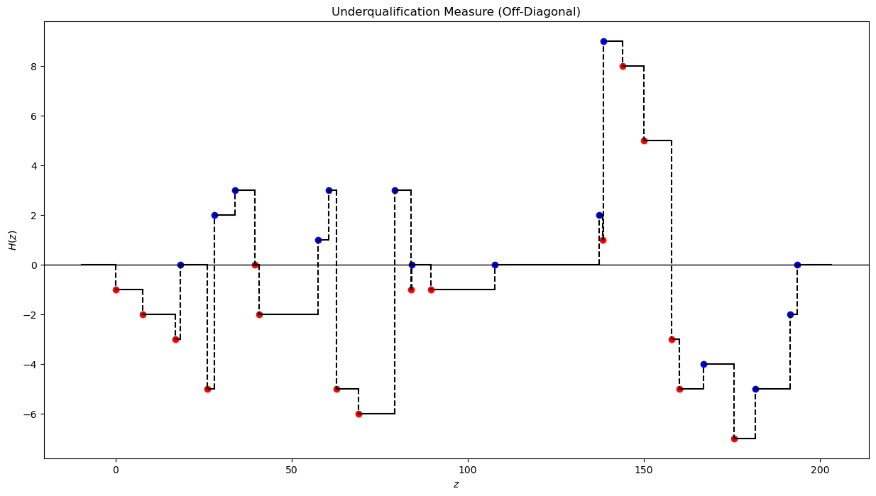
This suggests that the following quantity plays an important role:
Returning to our general (integer) discrete setting, let’s plot \(H\).
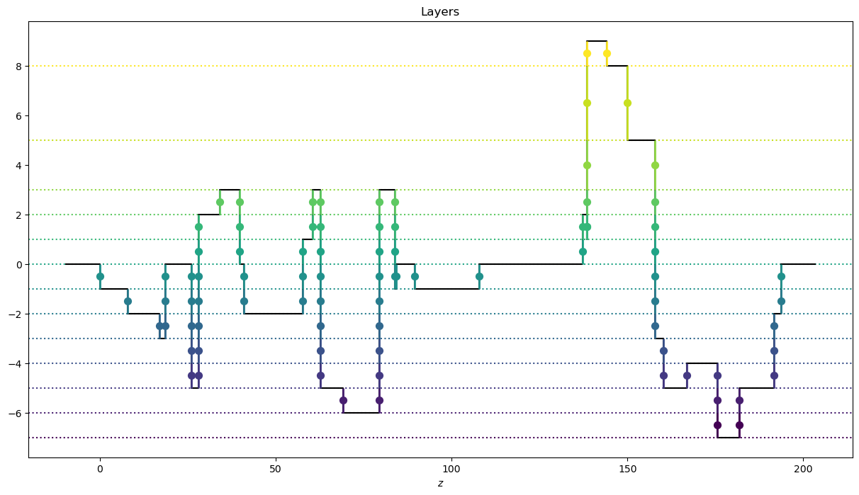
Notice that \(H\) is right-continuous (being the difference of right-continuous functions) and that upward (resp. downward) jumps correspond to point masses of agents with types from \(X\) (resp. \(Y\)).
def plot_H_z(self, figsize=(15, 8), range_x_axis=None, scatter=True):
    # Determine H(z) = F(z) - G(z)
    H_z = np.cumsum(self.q_z)

    # Plot H(z)
    plt.figure(figsize=figsize)
    plt.axhline(0, color='black', linewidth=1)

    # determine the step points for horizontal lines
    step = np.concatenate(([self.support_z.min() - .05 * np.ptp(self.support_z)],
                            self.support_z,
                           [self.support_z.max() + .05 * np.ptp(self.support_z)]))
    height = np.concatenate(([0], H_z, [0]))

    # plot the horizontal lines of the step function
    for i in range(len(step) - 1):
        plt.plot([step[i], step[i+1]], [height[i], height[i]], color='black')

    # draw dashed vertical lines for the step function
    for i in range(1, len(step) - 1):
        plt.plot([step[i], step[i]], [height[i-1], height[i]],
                color='black', linestyle='--')

    # plot discontinuities points of H(z)
    if scatter:
        plt.scatter(np.sort(self.X_types), H_z[self.q_z > 0], color='blue')
        plt.scatter(np.sort(self.Y_types), H_z[self.q_z < 0], color='red')

    if range_x_axis is not None:
        plt.xlim(range_x_axis)

    # Add labels and title
    plt.title('Underqualification Measure (Off-Diagonal)')
    plt.xlabel('$z$')
    plt.ylabel('$H(z)$')
    plt.grid(False)
    plt.gca().yaxis.set_major_locator(MaxNLocator(integer=True))
    plt.show()

OffDiagonal.plot_H_z = plot_H_z
example_off_diag.plot_H_z()
The layering property extends to the general discrete setting.
There are \(|H(\mathbb{R})|-1\) layers in total.
Enumerating the range of \(H\) as \(H(\mathbb{R}) = \{h_1,h_2, \dots, h_{|H(\mathbb{R})|}\}\) with \(h_1 < h_2 < \dots < h_{|H(\mathbb{R})|},\) we can define layer \(L_\ell,\) for \(\ell \in \{ 1,\dots,|H(\mathbb{R})|-1\}\) as the collection of types \(z \in Z\) such that
(which are types in \(X\)), or
which are types in \(Y\).
The mass associated with layer \(L_\ell\) is \(M_\ell = h_{\ell+1}- h_{\ell}.\)
Intuitively, a layer \(L_\ell\) consists of some mass \(M_\ell,\) of multiple types in \(Z,\) i.e. the problem within the layer is unitary.
A unitary problem is essentially an assignment problem up to a constant: we can solve the problem with unit mass and then rescale a solution by \(M_\ell.\)
Moreover, each layer \(L_\ell\) contains an even number of types \(N_\ell \in 2\mathbb{N},\) which are alternating, i.e., ordering them as \(z_1 < z_2\dots < z_{ N_\ell-1} < z_{ N_\ell}\) all odd (or even, respectively) indexed types belong to the same side.
The following method finds the layers associated with distributions \(F\) and \(G\).
Again, types in \(X\) are indexed with \(\{0, \dots,|X|-1\}\) and types in \(Y\) with \(\{|X|, \dots,|X| + |Y|-1\}\).
Using these indices (instead of the types themselves) to represent the layers allows keeping track of sides types in each layer, without adding an additional bit of information that would identify the side of the first type in the layer, which, because a layer is alternating, would then allow identifying sides of all types in the layer.
In addition, using indices will let us extract the cost function within a layer from the cost function \(c_{zz'}\) computed offline.
def find_layers(self):
    # Compute H(z) on the joint support
    H_z = np.concatenate([[0], np.cumsum(self.q_z)])

    # Compute the range of H, i.e. H(R), stored in ascending order
    layers_height = np.unique(H_z)

    # Compute the mass of each layer
    layers_mass = np.diff(layers_height)

    # Compute layers
    # the following |H(R)|x|Z| matrix has entry (z,l) equal to 1 iff type z belongs to layer l
    layers_01 = ((H_z[None, :-1] <= layers_height[:-1, None])
                 * (layers_height[1:, None] <= H_z[None, 1:]) |
                (H_z[None, 1:] <= layers_height[:-1, None])
                 * (layers_height[1:, None] <= H_z[None, :-1]))

    # each layer is reshaped as a list of indices corresponding to types
    layers = [self.type_z[layers_01[ell]]
                for ell in range(len(layers_height)-1)]

    return layers, layers_mass, layers_height, H_z

OffDiagonal.find_layers = find_layers
layers_list_example, layers_mass_example, _, _ = example_off_diag.find_layers()
print(layers_list_example)
[array([23, 10]), array([27, 3, 23, 10]), array([16, 2, 21, 3, 25, 8, 23, 12]), array([16, 2, 21, 3, 25, 12]), array([22, 0, 16, 2, 21, 3, 18, 12]), array([15, 0, 16, 2, 14, 5, 21, 3, 18, 9]), array([20, 0, 16, 2, 14, 5, 21, 3, 19, 11, 24, 1, 18, 9]), array([ 2, 26, 5, 21, 3, 19, 4, 18]), array([ 2, 26, 7, 21, 3, 19, 4, 17, 6, 18]), array([13, 26, 7, 21, 3, 19, 6, 18]), array([ 6, 18]), array([ 6, 28]), array([ 6, 29])]
The following method provides a graphical representation of the layers.
From the picture it is easy to spot two key features described above:
types are alternating
the layer problem is unitary
def plot_layers(self, figsize=(15, 8)):
    # Find layers
    layers, layers_mass , layers_height, H_z = self.find_layers()

    plt.figure(figsize=figsize)

    # Plot H(z)
    step = np.concatenate(([self.support_z.min() - .05 * np.ptp(self.support_z)],
                           self.support_z,
                           [self.support_z.max() + .05 * np.ptp(self.support_z)]))
    height = np.concatenate((H_z, [0]))
    plt.step(step, height, where='post', color='black', label='CDF', zorder=1)

    # Plot layers
    colors = cm.viridis(np.linspace(0, 1, len(layers)))
    for  ell, layer  in enumerate(layers):
        plt.vlines(self.types_list[layer], layers_height[ell] ,
                   layers_height[ell] + layers_mass[ell],
                   color=colors[ell], linewidth=2)
        plt.scatter(self.types_list[layer],
                    np.ones(len(layer)) * layers_height[ell]
                    +.5 * layers_mass[ell],
                    color=colors[ell], s=50)

        plt.axhline(layers_height[ell], color=colors[ell],
                    linestyle=':', linewidth=1.5, zorder=0)

    # Add labels and title
    plt.xlabel('$z$')
    plt.title('Layers')
    plt.gca().yaxis.set_major_locator(MaxNLocator(integer=True))
    plt.show()

OffDiagonal.plot_layers = plot_layers
example_off_diag.plot_layers()
16.3.2. Solving a layer#
Recall that layer \(L_\ell\) consists of a list of distinct types from \(Y \sqcup X\)
which is alternating.
The problem within a layer is unitary.
Hence we can solve the problem with unit masses and later rescale the solution by the layer’s mass \(M_\ell\).
Let us select a layer from the example above (we pick the one with maximum number of types) and plot the types on the real line
# Pick layer with maximum number of types
layer_id_example = max(enumerate(layers_list_example),
                    key = lambda x: len(x[1]))[0]
layer_example = layers_list_example[layer_id_example]


# Plot layer types
def plot_layer_types(self, layer, mass, figsize=(15, 3)):

    plt.figure(figsize=figsize)

    # Scatter plot n_x
    x_layer = layer[layer < len(self.X_types)]
    y_layer = layer[layer >= len(self.X_types)] - len(self.X_types)
    M_ell = np.ones(len(x_layer))* mass

    plt.scatter(self.X_types[x_layer], M_ell, color='blue', label='X types')
    plt.vlines(self.X_types[x_layer], ymin=0, ymax= M_ell,
               color='blue', linestyles='dashed')

    # Scatter plot m_y
    plt.scatter(self.Y_types[y_layer], - M_ell, color='red', label='Y types')
    plt.vlines(self.Y_types[y_layer], ymin=0, ymax=- M_ell,
               color='red', linestyles='dashed')

    # Add grid and y=0 axis
    # plt.grid(True)
    plt.axhline(0, color='black', linewidth=1)
    plt.gca().spines['bottom'].set_position(('data', 0))

    # Labeling the axes and the title
    plt.ylabel('mass')
    plt.title('Distributions of types in the layer')
    plt.gca().yaxis.set_major_locator(MaxNLocator(integer=True))
    plt.gca().spines['top'].set_visible(False)
    plt.gca().spines['right'].set_visible(False)
    plt.legend()
    plt.show()

ConcaveCostOT.plot_layer_types = plot_layer_types

example_off_diag.plot_layer_types(layer_example,
                                layers_mass_example[layer_id_example])

Given the structure of a layer and the no intersecting pairs property, the optimal matching and value of the layer can be found recursively.
Indeed, if in certain optimal matching \(1\) and \(j \in [N_\ell],\) \( j-1 \) odd, are paired, then there is no matching between agents in \([2,j-1]\) and those in \([j+1,N_\ell]\) (if both are non empty, i.e., \(j\) is not \(2\) or \(N_\ell\)).
Hence in such optimal solution agents in \([2,j-1]\) are matched among themselves.
Since \([z_2,z_{j-1}]\) (as well as \([z_{j+1},z_{N_\ell}]\)) is alternating, we can reason recursively.
Let \(V_{ij}\) be the optimal value of matching agents in \([i,j]\) with \(i,j \in [N_\ell],\) \(j -i \in \{1,3,\dots,N_\ell-1\}\).
Suppose that we computed the value \(V_{ij}\) for all \(i,j \in [N_\ell]\) with \(i-j \in \{1,3,\dots,t-2\}\) for some odd natural number \(t\).
Then for \(i,j \in [N_\ell]\) with \(i-j= t\)
with the RHS depending only on previously computed values.
We set the boundary conditions at \(t=-1\): \(V_{i+1,i} = 0\) for each \(i \in [N_\ell],\) so that we can apply the same Bellman equation (16.1) at \(t =1.\)
The following method takes as input the layer types indices and computes the value function as a matrix \([V_{ij}]_{ i \in [N_\ell+1], j \in [N_\ell ]}\).
In order to distinguish entries that are relevant for our computations from those that are never accessed, we initialize this matrix as full of NaN values.
def solve_bellman_eqs(self,layer):
    # Recover cost function within the layer
    cost_i_j = self.cost_z_z[layer[:,None],layer[None,:]]

    # Initialize value function
    V_i_j = np.full((len(layer)+1,len(layer)), np.nan)

    # Add boundary conditions
    i_bdry = np.arange(len(layer))
    V_i_j[i_bdry+1, i_bdry] = 0

    t = 1
    while t < len(layer):
        # Select agents i in [n_L-t] (with potential partners j's in [t,n_L])
        i_t = np.arange(len(layer)-t)

        # For each i, select each k with |k-i| <= t
        # (potential partners of i within segment)
        index_ik =  i_t[:,None] + np.arange(1, t+1, 2)[None,:]

        # Compute optimal value for pairs with |i-j| = t
        V_i_j[i_t, i_t + t] = (cost_i_j[i_t[:,None], index_ik] +
                                V_i_j[i_t[:,None] + 1, index_ik - 1] +
                                V_i_j[index_ik + 1, i_t[:,None] + t]).min(1)
        # Go to next odd integer
        t += 2

    return V_i_j

OffDiagonal.solve_bellman_eqs = solve_bellman_eqs
Let’s compute values for the layer from our example.
Only non-NaN entries are actually used in the computations.
# Compute layer value function
V_i_j = example_off_diag.solve_bellman_eqs(layer_example)

print(f"Type indices in the layer: {layer_example}")
print('##########################')
print("Section of the Value function of the layer:")
print(V_i_j.round(2)[:min(10, V_i_j.shape[0]),
                         :min(10, V_i_j.shape[1])])
Type indices in the layer: [20  0 16  2 14  5 21  3 19 11 24  1 18  9]
##########################
Section of the Value function of the layer:
[[  nan  4.29   nan  5.73   nan  9.82   nan 13.9    nan 14.52]
 [ 0.     nan  2.75   nan  6.17   nan  8.44   nan 10.56   nan]
 [  nan  0.     nan  1.44   nan  5.52   nan  9.6    nan 10.22]
 [  nan   nan  0.     nan  3.58   nan  5.84   nan  7.96   nan]
 [  nan   nan   nan  0.     nan  4.08   nan  8.16   nan  8.78]
 [  nan   nan   nan   nan  0.     nan  2.26   nan  4.38   nan]
 [  nan   nan   nan   nan   nan  0.     nan  4.08   nan  4.7 ]
 [  nan   nan   nan   nan   nan   nan  0.     nan  2.12   nan]
 [  nan   nan   nan   nan   nan   nan   nan  0.     nan  0.62]
 [  nan   nan   nan   nan   nan   nan   nan   nan  0.     nan]]
Policy evaluation
Having computed the value function, we can proceed to compute the optimal matching as the policy that attains the value function that solves the Bellman equation (16.1).
We start from agent \(1\) and match it with the \(k\) that achieves the minimum in the equation associated with \(V_{1,2N_\ell}.\)
Then we store segments \([2,k-1]\) and \([k+1,2N_\ell]\) (if not empty).
In general, given a segment \([i,j],\) we match \(i\) with \(k\) that achieves the minimum in the equation associated with \(V_{ij}\) and store the segments \([i,k-1]\) and \([k+1,j]\) (if not empty).
The algorithm proceeds until there are no segments left.
def find_layer_matching(self, V_i_j, layer):
    # Initialize
    segments_to_process  = [np.arange(len(layer))]
    matching = np.zeros((len(self.X_types),len(self.Y_types)), bool)

    while segments_to_process:
        # Pick i, first agent of the segment
        # and potential partners i+1,i+3,..., in the segment
        segment = segments_to_process[0]
        i_0 = segment[0]
        potential_matches = np.arange(i_0, segment[-1], 2) + 1

        # Compute optimal partner j_i
        obj = (self.cost_z_z[layer[i_0],layer[potential_matches]] +
                V_i_j[i_0 +1, potential_matches -1] +
                V_i_j[potential_matches +1,segment[-1]])

        j_i_0 = np.argmin(obj)*2 + (i_0 + 1)

        # Add matched pair (i,j_i)
        self.add_pair_to_matching(layer[[i_0,j_i_0]], matching)

        # Update segments to process:
        # remove current segment
        segments_to_process = segments_to_process[1:]

        # add [i+1,j-1] and [j+1,last agent of the segment]
        if j_i_0 > i_0 + 1:
            segments_to_process.append(np.arange(i_0 + 1, j_i_0))
        if j_i_0 < segment[-1]:
            segments_to_process.append(np.arange(j_i_0 + 1, segment[-1] + 1))

    return matching

OffDiagonal.find_layer_matching = find_layer_matching
Lets apply this method our example to find the matching within the layer and then rescale it by \(M_\ell\).
Note that the unscaled value equals \(V_{1,N_\ell}.\)
matching_layer = example_off_diag.find_layer_matching(V_i_j,layer_example)
print(f"Value of the layer (unscaled): {(matching_layer * example_off_diag.cost_x_y).sum()}")
print(f"Value of the layer (scaled by the mass = {layers_mass_example[layer_id_example]}): "
     f"{layers_mass_example[layer_id_example] * (matching_layer * example_off_diag.cost_x_y).sum()}")
Value of the layer (unscaled): 24.764959193288938
Value of the layer (scaled by the mass = 1): 24.764959193288938
The following method plots the matching within a layer.
We apply it to the layer from our example.
def plot_layer_matching(self, layer, matching_layer):
    # Create the figure and axis
    fig, ax = plt.subplots(figsize=(15, 15))

    # Plot the points on the x-axis
    X_types_layer = self.X_types[layer[layer < len(self.X_types)]]
    Y_types_layer = self.Y_types[layer[layer >= len(self.X_types)]
                    - len(self.X_types)]
    ax.scatter(X_types_layer, np.zeros_like(X_types_layer), color='blue',
                s = 20, zorder=5)
    ax.scatter(Y_types_layer, np.zeros_like(Y_types_layer), color='red',
                s = 20, zorder=5)

    # Draw semicircles for each row in matchings
    matched_types = np.where(matching_layer >0)
    matched_types_x = self.X_types[matched_types[0]]
    matched_types_y = self.Y_types[matched_types[1]]

    for iter in range(len(matched_types_x)):
        width = abs(matched_types_x[iter] - matched_types_y[iter])
        center = (matched_types_x[iter] + matched_types_y[iter]) / 2
        height = width
        semicircle = patches.Arc((center, 0), width, height, theta1=0,
                    theta2=180, lw=3)
        ax.add_patch(semicircle)

    # Add title and layout settings
    plt.title('Optimal Layer Matching' )
    ax.set_aspect('equal')
    plt.gca().spines['bottom'].set_position(('data', 0))
    ax.spines['left'].set_color('none')
    ax.spines['top'].set_color('none')
    ax.spines['right'].set_color('none')
    ax.yaxis.set_ticks([])
    ax.set_ylim(bottom= -np.ptp(self.support_z) / 100)

    plt.show()

ConcaveCostOT.plot_layer_matching = plot_layer_matching
example_off_diag.plot_layer_matching(layer_example, matching_layer)

16.3.2.1. Solving a layer in a smarter way#
We now present two key results in the context of OT with concave type costs.
We refer [Boerma et al., 2024] and [Delon et al., 2011] for proofs.
Consider the problem faced within a layer, i.e., types from \(Y \sqcup X\)
are alternating and the problem is unitary.
Given a matching on \([1,k],\) \(k \in [N_\ell],\) \(k\) even, we say that a matched pair \((i,j)\) within this matching is hidden if there is a matched pair \((i',j')\) with \(i' < i <j <j'.\)
Visually, the arc joining \((i',j')\) surmounts the arc joining \((i,j).\)
Theorem (DSS) Given an optimal matching on \([1,k],\) if \((i,j)\) is hidden in this matching, then the pair \((i,j)\) belongs to every optimal matching on \([1, 2 N_\ell]\) and is hidden in this matching too.
As a consequence, there exists a more efficient way to compute the value function within a layer.
It can be shown that the solving the following second-order difference equations delivers the same result as the Bellman equations (16.1) presented above:
for \(i,j \in [N_\ell],\) \(j-i\) odd, with boundary conditions \(V_{i+1,i}= 0\) for \(i \in [0,N_\ell ]\) and \(V_{i+2, i-1} = - c_{i,i+1}\) for \(i \in [N_\ell -1]\) .
The following method uses these equations to compute the value function that is stored as a matrix \([V_{ij}]_{ i \in [N_\ell+1], j \in [N_\ell +1]}.\)
def solve_bellman_eqs_DSS(self,layer):
    # Recover cost function within the layer
    cost_i_j = self.cost_z_z[layer[:,None],layer[None,:]]

    # Initialize value function
    V_i_j = np.full((len(layer)+1,len(layer)+1), np.nan)

    # Add boundary conditions
    V_i_j[np.arange(len(layer)+1), np.arange(len(layer)+1)] = 0
    i_bdry = np.arange(len(layer)-1)
    V_i_j[i_bdry+2,i_bdry] = - cost_i_j[i_bdry, i_bdry+1]

    t = 1
    while t < len(layer):
        # Select agents i in [n_l-t] and potential partner j=i+t for each i
        i_t = np.arange(len(layer)-t)
        j_t = i_t + t +1

        # Compute optimal values for ij with j-i = t
        V_i_j[i_t, j_t] = np.minimum(cost_i_j[i_t, j_t-1]
                        + V_i_j[i_t + 1, j_t - 1],
                        V_i_j[i_t, j_t - 2] + V_i_j[i_t + 2, j_t]
                        - V_i_j[i_t + 2, j_t - 2])

        ## Go to next odd integer
        t += 2

    return V_i_j

OffDiagonal.solve_bellman_eqs_DSS = solve_bellman_eqs_DSS
Let’s apply the algorithm to our example and compare outcomes with those attained with the Bellman equations above.
V_i_j_DSS = example_off_diag.solve_bellman_eqs_DSS(layer_example)

print(f"Type indices of the layer: {layer_example}")
print('##########################')

print("Section of Value function of the layer:")
print(V_i_j_DSS.round(2)[:min(10, V_i_j_DSS.shape[0]),
                         :min(10, V_i_j_DSS.shape[1])])

print('##########################')
print(f"Difference with previous Bellman equations: \
      {(V_i_j_DSS[:,1:] - V_i_j)[V_i_j >= 0].sum()}")
Type indices of the layer: [20  0 16  2 14  5 21  3 19 11 24  1 18  9]
##########################
Section of Value function of the layer:
[[ 0.     nan  4.29   nan  5.73   nan  9.82   nan 13.9    nan]
 [  nan  0.     nan  2.75   nan  6.17   nan  8.44   nan 10.56]
 [-4.29   nan  0.     nan  1.44   nan  5.52   nan  9.6    nan]
 [  nan -2.75   nan  0.     nan  3.58   nan  5.84   nan  7.96]
 [  nan   nan -1.44   nan  0.     nan  4.08   nan  8.16   nan]
 [  nan   nan   nan -3.58   nan  0.     nan  2.26   nan  4.38]
 [  nan   nan   nan   nan -4.08   nan  0.     nan  4.08   nan]
 [  nan   nan   nan   nan   nan -2.26   nan  0.     nan  2.12]
 [  nan   nan   nan   nan   nan   nan -4.08   nan  0.     nan]
 [  nan   nan   nan   nan   nan   nan   nan -2.12   nan  0.  ]]
##########################
Difference with previous Bellman equations:       4.440892098500626e-14
We can actually compute the optimal matching within the layer simultaneously with computing the value function, rather than sequentially.
The key idea is that, if at some step of the computation of the values the left branch of the minimum above achieves the minimum, say \(V_{ij}= c_{ij} + V_{i+1,j-1},\) then \((i,j)\) are optimally matched on \([i,j]\) and by the theorem above we get that a matching on \([i+1,j-1]\) which achieves \( V_{i+1,j-1}\) belongs to an optimal matching on the whole layer (since it is covered by the arc \((i,j)\) in \([i,j]\)).
We can therefore proceed as follows
We initialize an empty matching and a list with all the agents in the layer (representing the agents which are not matched yet).
Then whenever the left branch of the minimum is achieved for some \((i,j)\) in the computation of \(V,\) we take the collections of agents \(k_1,\dots,k_M\) in \([i+1,j-1]\) (in ascending order, i.e. with \(z_{k_{p}} < z_{k_{p+1}}\)) that are not matched yet (if any) and add to the matching the pairs \((k_1,k_2), (k_3,k_4),\dots,(k_{M-1},k_M).\)
Thus, we match each unmatched agent \(k_p\) in \([i+1,j-1]\) with the closest unmatched right neighbour \(k_{p+1}\) (starting from \(k_1\)).
Intuitively, if \(k_p\) were optimally matched with some \(k_{q}\) in \([i+1,j-1]\) and not with \(k_{p+1}\), then \(k_{p+1}\) would have already been hidden by the match \((k_p,k_{q})\) from some previous computation (because \(|k_p - k_q|< |i-j|\)) and it would therefore be matched.
Finally, if the process above leaves some umatched agents, we proceed by matching each of these agent with the closest unmatched right neighbour, starting again from the leftmost of these collection.
To gain understanding, note that this situation happens when the left branch is achieved only for pairs \(i,j\) with \(|i-j|=1,\) which leads to the optimal matching \((1,2), (2,3), \dots, (n_\ell -1, n_\ell).\)
def find_layer_matching_DSS(self,layer):
    # Recover cost function within the layer
    cost_i_j = self.cost_z_z[layer[:,None],layer[None,:]]

    # Add boundary conditions
    V_i_j = np.zeros((len(layer)+1,len(layer)+1))
    i_bdry = np.arange(len(layer)-1)
    V_i_j[i_bdry+2,i_bdry] = - cost_i_j[i_bdry, i_bdry+1]

    # Initialize matching and list of to-match agents
    unmatched = np.ones(len(layer), dtype = bool)
    matching = np.zeros((len(self.X_types),len(self.Y_types)), bool)

    t = 1
    while t < len(layer):
        # Compute optimal value for pairs with |i-j| = t
        i_t = np.arange(len(layer)-t)
        j_t = i_t + t + 1

        left_branch = cost_i_j[i_t, j_t-1] + V_i_j[i_t + 1, j_t - 1]
        V_i_j[i_t, j_t] = np.minimum(left_branch, V_i_j[i_t, j_t - 2]
                        + V_i_j[i_t + 2, j_t] - V_i_j[i_t + 2, j_t - 2])

        # Select each i for which left branch achieves minimum in the V_{i,i+t}
        left_branch_achieved = i_t[left_branch == V_i_j[i_t, j_t]]

        # Update matching
        for i in left_branch_achieved:
            # for each agent k in [i+1,i+t-1]
            for k in np.arange(i+1,i+t)[unmatched[range(i+1,i+t)]]:
                # if k is unmatched
                if unmatched[k] == True:
                    # find unmatched right neighbour
                    j_k = np.arange(k+1,len(layer))[unmatched[k+1:]][0]
                    # add pair to matching
                    self.add_pair_to_matching(layer[[k, j_k]], matching)
                    # remove pair from unmatched agents list
                    unmatched[[k, j_k]] = False

        # go to next odd integer
        t += 2

    # Each umatched agent is matched with next unmatched agent
    for i in np.arange(len(layer))[unmatched]:
        # if i is unmatched
        if unmatched[i] == True:
            # find unmatched right neighbour
            j_i = np.arange(i+1,len(layer))[unmatched[i+1:]][0]
            # add pair to matching
            self.add_pair_to_matching(layer[[i, j_i]], matching)
            # remove pair from unmatched agents list
            unmatched[[i, j_i]] = False

    return matching

OffDiagonal.find_layer_matching_DSS = find_layer_matching_DSS
matching_layer_DSS = example_off_diag.find_layer_matching_DSS(layer_example)
print(f" Value of layer with DSS recursive equations \
{(matching_layer_DSS * example_off_diag.cost_x_y).sum()}")
print(f" Value of layer with Bellman equations \
{(matching_layer * example_off_diag.cost_x_y).sum()}")
 Value of layer with DSS recursive equations 24.764959193288938
 Value of layer with Bellman equations 24.764959193288938
example_off_diag.plot_layer_matching(layer_example, matching_layer_DSS)

16.4. Solving primal problem#
The following method assembles our components in order to solve the primal problem.
First, if matches are perfect pairs, we store the on-diagonal matching and create an off-diagonal instance with the residual marginals.
Then we compute the set of layers of the residual distributions.
Finally, we solve each layer and put together matchings within each layer with the on-diagonal matchings.
We then return the full matching, the off-diagonal matching, and the off-diagonal instance.
def solve_primal_pb(self):
    # Compute on-diagonal matching, create new instance with residual types
    off_diagoff_diagonal, match_tuple = self.generate_offD_onD_matching()
    nonzero_id_x, nonzero_id_y, matching_diag = match_tuple

    # Compute layers
    layers_list, layers_mass, _, _ = off_diagoff_diagonal.find_layers()

    # Solve layers to compute off-diagonal matching
    matching_off_diag = np.zeros_like(off_diagoff_diagonal.cost_x_y, dtype=int)

    for ell, layer  in enumerate(layers_list):
        V_i_j = off_diagoff_diagonal.solve_bellman_eqs(layer)
        matching_off_diag += layers_mass[ell] \
                    * off_diagoff_diagonal.find_layer_matching(V_i_j, layer)

    # Add together on- and off-diagonal matchings
    matching = matching_diag.copy()
    matching[np.ix_(nonzero_id_x, nonzero_id_y)] += matching_off_diag

    return matching, matching_off_diag, off_diagoff_diagonal

ConcaveCostOT.solve_primal_pb = solve_primal_pb
matching, matching_off_diag, off_diagoff_diagonal = example_pb.solve_primal_pb()
We implement a similar method that adopts the DSS algorithm
def solve_primal_DSS(self):
    # Compute on-diagonal matching, create new instance with resitual types
    off_diagoff_diagonal, match_tuple = self.generate_offD_onD_matching()
    nonzero_id_x, nonzero_id_y, matching_diag = match_tuple

    # Find layers
    layers, layers_mass, _, _ = off_diagoff_diagonal.find_layers()

    # Solve layers to compute off-diagonal matching
    matching_off_diag = np.zeros_like(off_diagoff_diagonal.cost_x_y, dtype=int)

    for ell, layer  in enumerate(layers):
        matching_off_diag += layers_mass[ell] \
                          * off_diagoff_diagonal.find_layer_matching_DSS(layer)

    # Add together on- and off-diagonal matchings
    matching = matching_diag.copy()
    matching[np.ix_(nonzero_id_x, nonzero_id_y)] += matching_off_diag

    return matching, matching_off_diag, off_diagoff_diagonal

ConcaveCostOT.solve_primal_DSS = solve_primal_DSS
DSS_tuple = example_pb.solve_primal_DSS()
matching_DSS, matching_off_diag_DSS, off_diagoff_diagonal_DSS = DSS_tuple
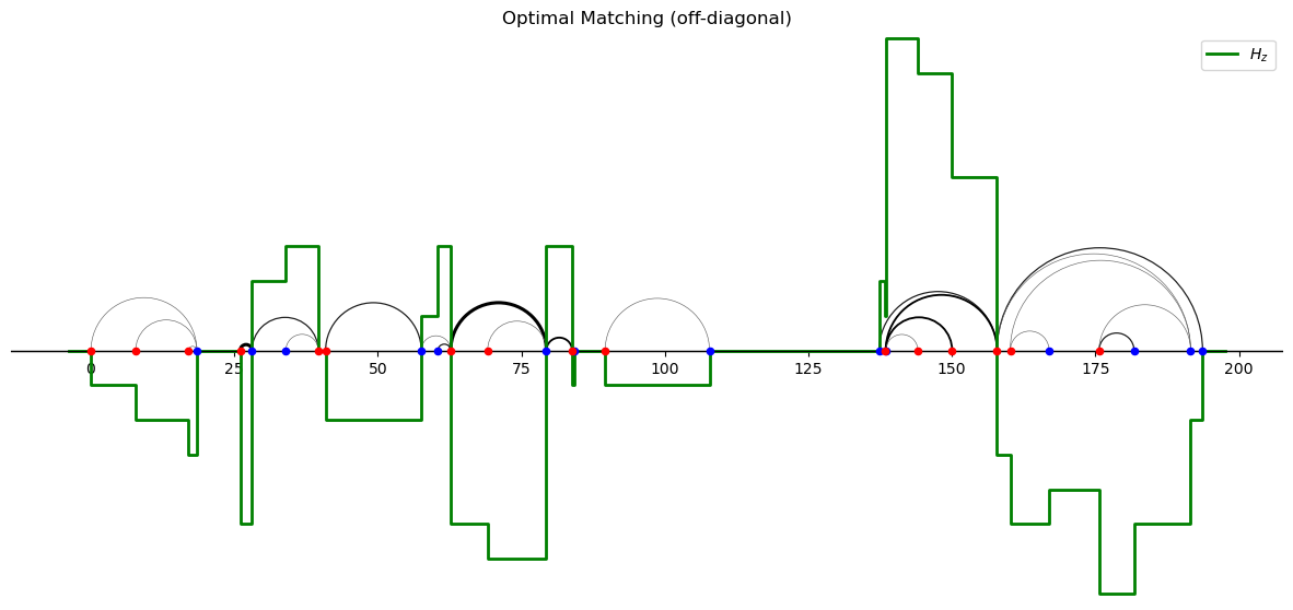
By drawing semicircles joining the matched agents (with distinct types), we can visualize the off-diagonal matching.
In the following figure, widths and colors of semicirles indicate relative numbers of agents that are “transported” along an arc.
def plot_matching(self, matching_off_diag, title, figsize=(15, 15),
                    add_labels=False, plot_H_z=False, scatter=True):

    # Create the figure and axis
    fig, ax = plt.subplots(figsize=figsize)

    # Plot types on the real line
    if scatter:
        ax.scatter(self.X_types, np.zeros_like(self.X_types), color='blue',
                    s=20, zorder=5)
        ax.scatter(self.Y_types, np.zeros_like(self.Y_types), color='red',
                    s=20, zorder=5)

    # Add labels for X_types and Y_types if add_labels is True
    if add_labels:
        # Remove x-axis ticks
        ax.set_xticks([])

        # Add labels
        for i, x in enumerate(self.X_types):
            ax.annotate(f'$x_{{{i }}}$', (x, 0), textcoords="offset points",
                        xytext=(0, -15), ha='center', color='blue', fontsize=12)
        for j, y in enumerate(self.Y_types):
            ax.annotate(f'$y_{{{j }}}$', (y, 0), textcoords="offset points",
                        xytext=(0, -15), ha='center', color='red', fontsize=12)

    # Draw semicircles for each pair of matched types
    matched_types = np.where(matching_off_diag > 0)
    matched_types_x = self.X_types[matched_types[0]]
    matched_types_y = self.Y_types[matched_types[1]]

    count = matching_off_diag[matched_types]
    colors = plt.cm.Greys(np.linspace(0.5, 1.5, count.max() + 1))
    max_height = 0
    for iter in range(len(count)):
        width = abs(matched_types_x[iter] - matched_types_y[iter])
        center = (matched_types_x[iter] + matched_types_y[iter]) / 2
        height = width
        max_height = max(max_height, height)
        semicircle = patches.Arc((center, 0), width, height,
                                 theta1=0, theta2=180,
                                 color=colors[count[iter]],
                                 lw=count[iter] * (2.2 / count.max()))
        ax.add_patch(semicircle)

    # Title and layout settings for the main plot
    plt.title(title)
    ax.set_aspect('equal')
    plt.axhline(0, color='black', linewidth=1)
    ax.spines['bottom'].set_position(('data', 0))
    ax.spines['left'].set_color('none')
    ax.spines['top'].set_color('none')
    ax.spines['right'].set_color('none')
    ax.yaxis.set_ticks([])
    ax.set_ylim(- np.ptp(self.X_types) / 10,
                (max_height / 2) + np.ptp(self.X_types)*.01)

    # Plot H_z on the main axis if enabled
    if plot_H_z:
        H_z = np.cumsum(self.q_z)

        step = np.concatenate(([self.support_z.min()
                                - .02 * np.ptp(self.support_z)],
                                self.support_z,
                                [self.support_z.max()
                                + .02 * np.ptp(self.support_z)]))

        H_z = H_z/np.ptp(H_z) * np.ptp(self.support_z) /2
        height = np.concatenate(([0], H_z, [0]))

        # Plot the compressed H_z on the same main x-axis
        ax.step(step, height, color='green', lw=2,
                                label='$H_z$', where='post')

        # Set the y-limit to keep H_z and maximum circle size in the plot
        ax.set_ylim(np.min(H_z) - np.ptp(H_z) *.01,
                    np.maximum(np.max(H_z), max_height / 2) + np.ptp(H_z) *.01)

        # Add label and legend for H_z
        ax.legend(loc="upper right")

        plt.show()

ConcaveCostOT.plot_matching = plot_matching
off_diagoff_diagonal.plot_matching(matching_off_diag,
            title='Optimal Matching (off-diagonal)', plot_H_z=True)
off_diagoff_diagonal_DSS.plot_matching(matching_off_diag_DSS,
            title='Optimal Matching (off-diagonal) with DSS algorithm')

16.4.1. Verify with linear programming#
Let’s verify some of the proceeding findings using linear programming.
def solve_1to1(c_i_j, n_x, m_y, return_dual=False):
    n, m = np.shape(c_i_j)

    # Constraint matrix
    M_z_a = np.vstack([np.kron(np.eye(n), np.ones(m)),
                       np.kron(np.ones(n), np.eye(m))])
    # Constraint vector
    q = np.concatenate((n_x, m_y))

    # Solve the linear programming problem using linprog from scipy
    result = linprog(c_i_j.flatten(), A_eq=M_z_a, b_eq=q,
                        bounds=(0, None), method='highs')

    if return_dual:
        return (np.round(result.x).astype(int).reshape([n, m]),
                result.eqlin.marginals)
    else:
        return np.round(result.x).astype(int).reshape([n, m])
mu_x_y_LP = solve_1to1(example_pb.cost_x_y,
                example_pb.n_x,
                example_pb.m_y)
print(f"Value of LP (scipy): {(mu_x_y_LP * example_pb.cost_x_y).sum()}")
print(f"Value (plain Bellman equations): {(matching * example_pb.cost_x_y).sum()}")
print(f"Value (DSS): {(matching_DSS * example_pb.cost_x_y).sum()}")
Value of LP (scipy): 143.45490363125705
Value (plain Bellman equations): 143.45490363125705
Value (DSS): 143.45490363125705
16.5. Examples#
16.5.1. Example 1#
We study optimal transport problems on the real line with cost \(c(x,y)= h(|x-y|)\) for a strictly concave and increasing function \(h: \mathbb{R}_+ \rightarrow \mathbb{R}_+.\)
The outcome is called composite sorting.
Here, we will focus on \(c(x,y)=|x-y|^{\frac{1}{\zeta}}\) for \(\zeta>1\)
To appreciate differences with positive assortative matching (PAM) note that the latter is induced by a cost of the form \( h(x-y)\) for some strictly convex \(h: \mathbb{R} \rightarrow \mathbb{R}_+.\)
See Santambrogio 2015, Ch. 2.2.
For example, the cost function \(|x-y|^{p},p>1\) induces PAM.
On the other hand, negative assortative matching (NAM) arises if \(c(x,y)= h(x-y)\) with \(h: \mathbb{R} \rightarrow \mathbb{R}_+\) strictly concave.
For example, the cost function \(-|x-y|^{p},p>1,\) induces NAM.
Thus, NAM corresponds to a matching that maximizes a transport problem criterion with gain function \(g(x,y)=|x-y|^{p}\).
Note how PAM and NAM differ from composite sorting
Composite sorting is induced by a cost that is the composition of a strictly concave increasing function \(h\) and a convex function \(|\cdot|\) applied to displacement \(x-y.\)
Different functions \(h\) potentially induce different matchings.
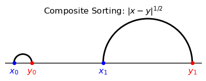
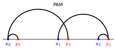
The following example shows that composite matching can feature both positive and negative assortative patterns.
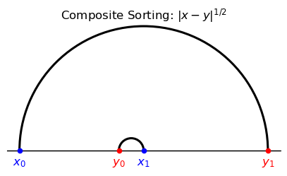
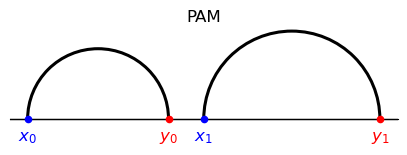
Suppose that there are two agents per side and types
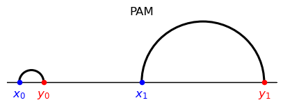
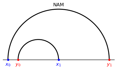
There are two feasible matchings, one corresponding to PAM, the other to NAM.
The first features two displacements \(|\textcolor{blue}{x_0} - \textcolor{red}{y_0}| ,| \textcolor{blue}{x_1} - \textcolor{red}{y_1}|\)
The second features a large displacement \(|\textcolor{blue}{x_0} - \textcolor{red}{y_1}| \) and a small displacement \(| \textcolor{blue}{x_1} - \textcolor{red}{y_0}|.\)
Evidently,
PAM corresponds to the matching with two medium side displacement because the correponding cost is strictly convex and increasing in the displacement.
NAM corresponds to the matching with a small displacement and a large displacement because the gain is strictly convex and increasing in the displacement.
In this example, composite sorting ends up coinciding with NAM, but this is something of a coincidence
Thus, note that in composite matching the cost function is strictly concave and increasing in the displacement.
N = 2
p = 2
ζ = 2

# Solve composite sorting problem
example_1 = ConcaveCostOT(np.array([0,5]),
                          np.array([4,10]),
                          ζ=ζ)
matching_CS, _ ,_ = example_1.solve_primal_DSS()

# Solve PAM and NAM
# I use the linear programs to compute PAM and NAM,
# but of course they can be computed directly

convex_cost = np.abs(example_1.X_types[:,None] - example_1.Y_types[None,:])**p

#PAM: |x-y|^p , p>1
matching_PAM = solve_1to1(convex_cost, example_1.n_x, example_1.m_y)

#NAM: -|x-y|^p , p>1
matching_NAM = solve_1to1(-convex_cost, example_1.n_x, example_1.m_y)

# Plot the matchings
example_1.plot_matching(matching_CS,
                title=f'Composite Sorting: $|x-y|^{{1/{ζ}}}$',
                figsize=(5,5), add_labels=True)
example_1.plot_matching(matching_PAM, title='PAM',
                figsize=(5,5), add_labels=True)
To explore the coincidental resemblence to a NAM outcome, let’s shift left type \(\textcolor{red}{y_0} \) while keeping it in between \(\textcolor{blue}{x_0}\) and \(\textcolor{blue}{x_1}\).
PAM and NAM are invariant to any such shift.
However, for a large enough shift, composite sorting now coincides with PAM.
N = 2
ζ = 2
p = 2

# Solve composite sorting problem
example_1 = ConcaveCostOT(np.array([0,5]),
                          np.array([1,10]) ,
                           ζ = ζ)
matching_CS, _ ,_ = example_1.solve_primal_DSS()

# Solve PAM and NAM
convex_cost = np.abs(example_1.X_types[:,None] - example_1.Y_types[None,:])**p

matching_PAM = solve_1to1(convex_cost, example_1.n_x, example_1.m_y)
matching_NAM = solve_1to1(-convex_cost, example_1.n_x, example_1.m_y)

# Plot the matchings
example_1.plot_matching(matching_CS,
        title = f'Composite Sorting: $|x-y|^{{1/{ζ}}}$',
        figsize = (5,5), add_labels = True)
example_1.plot_matching(matching_PAM, title = 'PAM',
        figsize = (5,5), add_labels = True)
example_1.plot_matching(matching_NAM, title = 'NAM',
        figsize = (5,5), add_labels = True)
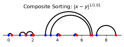
Finally, notice that the Monge problem cost function \(|x-y|\) equals the limit of the composite sorting cost \(|x-y|^{1/\zeta}\) as \(\zeta \downarrow 1\) and also the limit of \(|x-y|^p\) as \(p \downarrow 1.\)
Evidently, the Monge problem is solved by both the PAM and the composite sorting assignment that arises for \(\zeta \downarrow 1.\)
In the following example, the Monge cost of the composite sorting assignment equals the Monge cost of PAM.
Consequently, it is optimal for the Monge problem.
N = 10

ζ = 1.01
p = 2
np.random.seed(1)
X_types = np.random.uniform(0,10, size=N)
Y_types = np.random.uniform(0,10, size=N)

# Solve composite sorting problem
example_1 = ConcaveCostOT(X_types, Y_types, ζ=ζ)

matching_CS, _ ,_ = example_1.solve_primal_DSS()

# Solve PAM and NAM
convex_cost = np.abs(X_types[:,None] - Y_types[None,:])** p

matching_PAM = solve_1to1(convex_cost, example_1.n_x, example_1.m_y)
matching_NAM = solve_1to1(-convex_cost, example_1.n_x, example_1.m_y)


example_1.plot_matching(matching_CS,
            title=f'Composite Sorting: $|x-y|^{{1/{ζ}}}$', figsize=(5,5))
example_1.plot_matching(matching_PAM, title = 'PAM', figsize=(5,5))

monge_cost_comp = (matching_CS * np.abs(X_types[:,None] - Y_types[None,:])).sum()
monge_cost_PAM = (matching_PAM * np.abs(example_1.X_types[:,None]
                               - example_1.Y_types[None,:])).sum()
print("Monge cost of the composite matching assignment:")
print(monge_cost_comp)
print("Monge cost of PAM:")
print(monge_cost_PAM)
Monge cost of the composite matching assignment:
10.530287849572634
Monge cost of PAM:
10.530287849572636

16.5.2. Example 2#
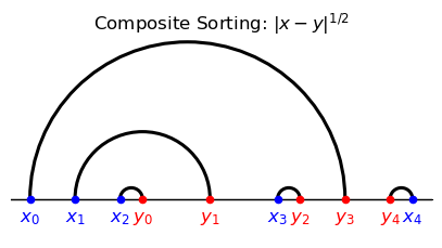
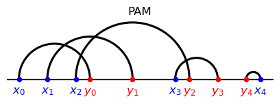
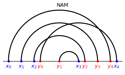
The following example has five agents per side.
The composite sorting assignment differs from both PAM and NAM.
Composite sorting features a hierarchical structure, with each hierarchy positively sorted.
Indeed, consider the composite sorting assignment and note that
the only arcs visible from above are the ones corresponding to pairings \((\textcolor{blue}{x_0},\textcolor{red}{y_3})\) and \((\textcolor{red}{y_4},\textcolor{blue}{x_4});\)
after removing these agents, the only arcs visible from above correspond to \((\textcolor{blue}{x_1},\textcolor{red}{y_1})\) and \((\textcolor{blue}{x_3},\textcolor{red}{y_2})\) ;
after removing these agents, the only arc/pairing left is \((\textcolor{blue}{x_2},\textcolor{red}{y_0}).\)
Note that, at each iteration, the partial assignment corresponding to the arcs visible from above features positive assortativeness.
Another distinct feature of composite matching stands out from the figures:
arcs do not intersect
N = 5
ζ = 2
p = 2

X_types_example_2 = np.array([-2,0,2,9, 15])
Y_types_example_2 = np.array([3,6,10,12, 14])

# Solve composite sorting problem
example_2 = ConcaveCostOT(X_types_example_2, Y_types_example_2, ζ=ζ)

matching_CS, _ ,_ = example_2.solve_primal_DSS()

# Solve PAM and NAM
convex_cost = np.abs(X_types_example_2[:,None] - Y_types_example_2[None,:])** p

matching_PAM = solve_1to1(convex_cost, example_2.n_x, example_2.m_y)
matching_NAM = solve_1to1(-convex_cost, example_2.n_x, example_2.m_y)


example_2.plot_matching(matching_CS, title = 'Composite Sorting: $|x-y|^{1/2}$',
                        figsize = (5,5), add_labels=True)
example_2.plot_matching(matching_PAM, title = 'PAM',
                        figsize = (5,5), add_labels=True)
example_2.plot_matching(matching_NAM, title = 'NAM',
                        figsize = (5,5), add_labels=True)
16.5.3. Example 3#
[Boerma et al., 2024] provide the following example.
There are four agents per side and three types per side (so the problem is not unitary, as opposed to the examples above).
X_types_example_3 = np.array([0,5,9])
Y_types_example_3 = np.array([1,6,10])
n_x_example_3 =  np.array([2,1,1], dtype= int)
m_y_example_3 =  np.array([1,1,2], dtype= int)


example_3 = ConcaveCostOT(X_types_example_3, Y_types_example_3,
                          n_x_example_3, m_y_example_3, ζ = 2)
example_3.plot_marginals(figsize = (5,5))
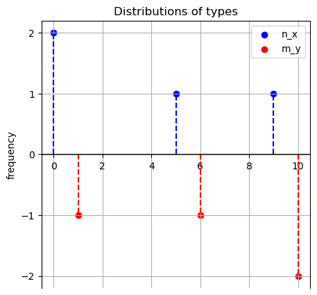
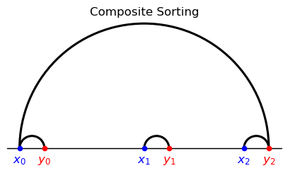
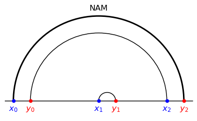
In the case of positive assortative matching (PAM), the two agents with lowest value \(\textcolor{blue}{x_0} \) are matched with the lowest valued agents on the other side \(\textcolor{red}{y_0},\textcolor{red}{y_1}.\)
Similarly, the agents with highest value \(\textcolor{red}{y_2} \) are matched with the highest valued types on the other side, \(\textcolor{blue}{x_1}\) and \(\textcolor{blue}{x_2}. \)
Composite sorting features both negative and positive sorting patterns: agents of type \(\textcolor{blue}{x_0}\) are matched with both the bottom \(\textcolor{red}{y_0}\) and the top \(\textcolor{red}{y_2}\) of the distribution.
matching_CS, _ ,_ = example_3.solve_primal_DSS()

convex_cost = np.abs(example_3.X_types[:,None] - example_3.Y_types[None,:])**2
matching_PAM = solve_1to1(convex_cost, example_3.n_x, example_3.m_y)
matching_NAM = solve_1to1(-convex_cost, example_3.n_x, example_3.m_y)

example_3.plot_matching(matching_PAM, title = 'PAM',
                        figsize = (5,5), add_labels= True)
example_3.plot_matching(matching_CS, title = 'Composite Sorting',
                        figsize = (5,5), add_labels= True)
example_3.plot_matching(matching_NAM, title = 'NAM',
                        figsize = (5,5), add_labels= True)
16.6. Dual solution#
Let’s recall the formulation
The dual problem is
where \((\phi , \psi) \) are dual variables, which can be interpreted as shadow cost of agents in \(X\) and \(Y\), respectively.
Since the dual is feasible and bounded, \(V_P = V_D\) (strong duality prevails).
Assume now that \(y_{xy} = \alpha_x + \gamma_y - c_{xy}\) is the output generated by matching \(x\) and \(y.\)
It includes the sum of \(x\) and \(y\) specific amenities/outputs minus the cost \(c_{xy}.\)
Then we can formulate the following problem and its dual
Given the constraints, the primal problem \(W_P\) does not depend on \(\alpha,\gamma\) and it has the same solutions as the cost minimization problem \(V_P\).
The values are related by \(W_P = \sum_{x \in X}n_x \alpha_x + \sum_{y \in Y}m_y \gamma_y - V_P.\)
The dual solutions of \(V_D\) and \(W_D\) are related by \(u_x = \alpha_x - \phi_x\) and \(v_y = \gamma_y - \psi_y.\)
The dual solution \((u,v)\) of \(W_D\) can be interpreted as equilibrium utilities of the agents, which include the individual specific amenities and equilibrium shadow costs.
[Boerma et al., 2024] propose an efficient method to compute the dual variables from the optimal matching (primal solution) in the case of composite sorting.
Their approach relies on Complementary Slackness: given a primal solution \(\mu\), \((\phi , \psi) \) is a dual solution if and only if for all \(x \in X\) and \(y \in Y\)
\(\phi_x + \psi_y \leq c_{xy}\) (dual feasibility),
\(\phi_x + \psi_y = c_{xy}\) if \(\mu_{xy}>0\) (complementary slackness).
Let’s generate an instance and compute the optimal matching.
num_agents = 8

np.random.seed(1)

X_types_assignment_pb = np.random.uniform(0, 10, size=num_agents)
Y_types_assignment_pb = np.random.uniform(0, 10, size=num_agents)


# Create instance of the problem
exam_assign = ConcaveCostOT(X_types_assignment_pb, Y_types_assignment_pb)

# Solve primal problem
assignment, assignment_OD, exam_assign_OD = exam_assign.solve_primal_DSS()

# Plot matching
add_labels = True if num_agents < 16 else False
exam_assign_OD.plot_matching(assignment_OD, title = f'Composite Sorting',
                            figsize=(10,10), add_labels=add_labels)
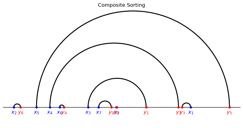
Having computed the optimal matching, we say that a pair \((x_0,y_0)\) is a subpair of a matched pair \((x,y)\) if \(x_0,y_0\) are in the open interval between \(x\) and \(y\) and the pair \((x_0,y_0)\) is not nested.
The following method computes the subpairs of the optimal matching of the off-diagonal instance.
The output of this method is a dictionary with keys corresponding to matched pairs and an “artificial pair” which collects all arcs which are visible from above.
Values of each key \((x_0,y_0)\) are the subpairs ordered so that the first subpair is the subpair with the \(x\) type closest to \(x_0\) and the last subpair is the subpair with the \(y\) type closest to \(y_0.\)
def sort_subpairs(self, subpairs, x_smaller_y=True ):

    x_key = min if x_smaller_y else max
    y_key = max if x_smaller_y else min

    first_pair = x_key(subpairs, key=lambda pair: self.X_types[pair[0]])
    last_pair = y_key(subpairs, key=lambda pair: self.Y_types[pair[1]])

    intermediate_pairs = [pair for pair in subpairs
                            if pair != first_pair and pair != last_pair]

    return [first_pair] + intermediate_pairs + [last_pair]

ConcaveCostOT.sort_subpairs = sort_subpairs

def find_subpairs(self, matching, return_pairs_between = False):

    # Create set of matched pairs of types and add an artificial pair
    matched_pairs = set( zip(* np.where(matching > 0)))

    # Initialize dictionary to store subpairs
    subpairs = {}
    pairs_between = {}

    # Find subpairs (both nested and non-nested) for each matched pair
    for matched_pair in matched_pairs | {'artificial_pair'}:
        # Determine the interval of the matched pair
        if matched_pair != 'artificial_pair':
            min_type, max_type = sorted([self.X_types[matched_pair[0]],
                                         self.Y_types[matched_pair[1]]])
        else:
            min_type, max_type = (-np.inf, np.inf)

        # Add all pairs in the interval to the list of nested_subpairs
        pairs_between[matched_pair] = {
                    pair for pair in matched_pairs if pair != matched_pair and
                    min_type <= self.X_types[pair[0]] <= max_type and
                    min_type <= self.Y_types[pair[1]] <= max_type}

    subpairs = {key: value.copy() for key, value in pairs_between.items()}

    # Remove nested pairs
    for matched_pair in matched_pairs | {'artificial_pair'}:
        # Compute all nested subpairs
        nested_subpairs = set(chain.from_iterable(subpairs[pair]
                                for pair in subpairs[matched_pair]))
        # Remove nested pairs from subpairs[matched_pair]
        subpairs[matched_pair] -= nested_subpairs
        # subpairs[matched_pair].discard(matched_pair)
        subpairs[matched_pair] = list(subpairs[matched_pair])

        # Order the subpairs:
        # the first (last) pair should have x (y) close to pair_x (pair_y)
        if matched_pair != 'artificial_pair' and len(subpairs[matched_pair]) > 1:
            subpairs[matched_pair] = self.sort_subpairs(
                subpairs[matched_pair],
                x_smaller_y=self.X_types[matched_pair[0]]
                            < self.Y_types[matched_pair[1]])

    if return_pairs_between:
        return subpairs, pairs_between
    return subpairs

OffDiagonal.find_subpairs = find_subpairs
subpairs, pairs_between = exam_assign_OD.find_subpairs(assignment,
                                                return_pairs_between = True)
subpairs
{(np.int64(5), np.int64(5)): [(np.int64(4), np.int64(7)),
  (np.int64(1), np.int64(3))],
 'artificial_pair': [(np.int64(5), np.int64(5)), (np.int64(2), np.int64(6))],
 (np.int64(3), np.int64(1)): [(np.int64(7), np.int64(0)),
  (np.int64(0), np.int64(2))],
 (np.int64(7), np.int64(0)): [],
 (np.int64(6), np.int64(4)): [],
 (np.int64(0), np.int64(2)): [],
 (np.int64(2), np.int64(6)): [],
 (np.int64(1), np.int64(3)): [],
 (np.int64(4), np.int64(7)): [(np.int64(6), np.int64(4)),
  (np.int64(3), np.int64(1))]}
The algorithm to compute the dual variables has a hierarchical structure: it starts from the matched pairs with no subpairs and then moves to those pairs whose subpairs have been already processed.
We can visualize the hierarchical structure by computing the order in which he pairs will be processed and plotting the matching with color of the arcs corresponding the hierarchy.
## Compute hierarchies

def find_hierarchies(subpairs):

    # Initialize sets for faster membership checks
    pairs_to_process = set(subpairs.keys())  # All pairs to process
    processed_pairs = set()  # Pairs that have been processed

    # Initialize ready_to_process with pairs that have no subpairs
    ready_to_process = {pair for pair, sublist in subpairs.items()
                        if len(sublist) == 0}

    # Initialize hierarchies with the first level
    hierarchies = [list(ready_to_process)]

    # Continue processing while there are unprocessed pairs
    while len(processed_pairs) < len(subpairs):
        # Mark ready_to_process pairs as processed
        processed_pairs.update(ready_to_process)

        # Remove ready_to_process pairs from pairs_to_process
        pairs_to_process -= ready_to_process

        # Find new ready_to_process pairs that have all their subpairs processed
        ready_to_process = {
            pair for pair in pairs_to_process
            if all(subpair in processed_pairs for subpair in subpairs[pair])}

        # Append the new ready_to_process to hierarchies
        hierarchies.append(list(ready_to_process))

    return hierarchies

## Plot hierarchies

def plot_hierarchies(self, subpairs, scatter=True, range_x_axis=None):
    # Compute hierarchies
    hierarchies = find_hierarchies(subpairs)

    # Create the figure and axis
    fig, ax = plt.subplots(figsize=(15, 15))

    # Plot types on the real line (blue for X_types, red for Y_types)
    size_marker = 20 if scatter else 0
    ax.scatter(self.X_types, np.zeros_like(self.X_types), color='blue',
                    s=size_marker, zorder=5, label='X_types')
    ax.scatter(self.Y_types, np.zeros_like(self.Y_types), color='red',
                    s=size_marker, zorder=5, label='Y_types')

    # Plot arcs
    # Create a colormap ('viridis' or 'coolwarm', 'plasma')
    cmap = plt.colormaps['plasma']
    for level, hierarchy in enumerate(hierarchies):
        color = (cmap(level / (len(hierarchies) - 1))
                        if len(hierarchies) > 1 else cmap(0))
        for pair in hierarchy:
            if pair == 'artificial_pair':
                continue

            min_type, max_type = sorted([self.X_types[pair[0]],
                                         self.Y_types[pair[1]]])
            width = max_type - min_type
            center = (max_type + min_type) / 2
            # Semicircle height can be the same as the width for a perfect arc
            height = width
            semicircle = patches.Arc((center, 0), width, height,
                            theta1=0, theta2=180,
                            color=color, lw = 3)
            ax.add_patch(semicircle)

    if range_x_axis is not None:
        ax.set_xlim(range_x_axis)
        ax.set_ylim(- np.ptp(self.X_types) / 10,
                    (range_x_axis[1] - range_x_axis[0]) / 2 )

    # Title and layout settings for the main plot
    plt.title('Hierarchies of the optimal matching (off-diagonal)')
    ax.set_aspect('equal')
    plt.axhline(0, color='black', linewidth=1)
    ax.spines['bottom'].set_position(('data', 0))
    ax.spines['left'].set_color('none')
    ax.spines['top'].set_color('none')
    ax.spines['right'].set_color('none')
    ax.yaxis.set_ticks([])  # Hide the y-axis ticks

    # Add a colorbar to represent hierarchy levels
    sm = cm.ScalarMappable(cmap=cmap,
                    norm=Normalize(vmin=0, vmax= len(hierarchies) - 1))
    sm.set_array([])
    cbar = plt.colorbar(sm, ax=ax, orientation='vertical', pad=0.1, shrink=0.2)
    # Show only min and max levels
    cbar.set_ticks([0, len(hierarchies) - 1])
    # Label the ticks for clarity
    cbar.set_ticklabels(['Lowest', 'Highest'])

    plt.show()

OffDiagonal.plot_hierarchies = plot_hierarchies
exam_assign_OD.plot_hierarchies(subpairs)
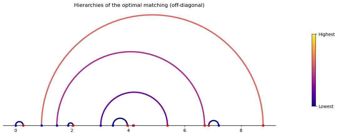
We proceed to describe and implement the algorithm to compute the dual solution.
As already mentioned, the algorithm starts from the matched pairs \((x_0,y_0)\) with no subpairs and assigns the (temporary) values \(\phi_{x_0} = c_{x_0 y_0}\) and \(\psi_{y_0} = 0,\) i.e. the \(x\) type sustains the whole cost of matching.
The algorithm then proceeds sequentially by processing any matched pair whose subpairs have already been processed.
After picking any such matched pair \((x_0,y_0)\), the dual variables already computed for the processed subpairs need to be made “comparable”.
Indeed, for any subpair \((x_1,y_1)\) of \((x_0,y_0)\), the dual variables of all the types between the \(x_1\) and \(y_1\) satisfy dual feasibility and complementary slackness locally, i.e. \(\phi_x + \psi_y \leq c_{xy}\) with equality if \((x,y)\) is a matched pair for all types \(x,y\) between \(x_0\) and \(y_0.\)
But dual feasibility is not satisfied globally in general, for instance it might not be satisfied for two subpairs \((x_1,y_1)\) and \((x_2,y_2)\) of \((x_0,y_0).\)
Therefore, letting \((x_1,y_1), \dots, (x_p,y_p)\) be the subpairs of \((x_0,y_0),\) we compute the solution \((\beta_2, \dots, \beta_p) \) of the linear system
Then for all \(i \in [p]\) compute the adjustment \( \Delta_i = \sum_{k = i+1}^p \beta_k + \phi_{x_p} - \phi_{x_i}\) and modify the dual variables
for all matched pairs \((x,y)\) between \(x_i\) and \(y_i.\)
After this step, the dual variables of the types between \(x_0\) and \(y_0\) satisfy dual feasibility and complementary slackness; we can then proceed to compute the dual variables for \(x_0\) and \(y_0\) by setting
The pair \((x_0,y_0)\) is now processed.
The following method computes the solution \(\beta\) of the linear system of inequalities above.
def compute_betas(self, pair, subpairs):
    types_subpairs = np.array(subpairs)

    # Define the bounds of the linear inequality system
    if pair == 'artificial_pair':
        bounds = (- self.cost_x_y[types_subpairs[:,0][:,None],
                types_subpairs[:,1][None,:]]
                + self.cost_x_y[types_subpairs[:,0],
                                types_subpairs[:,1]][None,:])
    else:
        bounds = (np.maximum(
        self.cost_x_y[pair]
        - self.cost_x_y[pair[0], types_subpairs[:,1]][None,:]
        - self.cost_x_y[types_subpairs[:,0],pair[1]][:,None],
        - self.cost_x_y[types_subpairs[:,0][:,None],
        types_subpairs[:,1][None,:]]
        )
        + self.cost_x_y[types_subpairs[:,0], types_subpairs[:,1]][None,:])

    # Define linear inequality system
    num_subpairs = len(types_subpairs)
    c_1 = (np.arange(num_subpairs)[:, None, None]
            >= np.arange(num_subpairs)[None, None, :])
    c_2 = (np.arange(num_subpairs)[None, None, :]
            > np.arange(num_subpairs)[ None,:, None])
    sum_tensor = (c_1 & c_2).astype(int)

    sum_tensor -= sum_tensor.transpose(1, 0, 2)

    # Solve the system of linear inequalities
    result = linprog(c = np.zeros(num_subpairs),
                    A_ub= - sum_tensor.reshape(num_subpairs**2, num_subpairs),
                    b_ub= - bounds.flatten(),
                    bounds=(None,None),
                    method='highs')

    beta = result.x
    beta[0] = 0

    return beta

OffDiagonal.compute_betas = compute_betas
The following method iteratively processes the matched pairs of the off-diagonal matching as explained above.
def compute_dual_off_diagonal(self, subpairs, pairs_between):

    # Initialize dual variables
    ϕ_x = np.zeros(len(self.X_types))
    ψ_y = np.zeros(len(self.Y_types))

    # Initialize sets for faster membership checks
    pairs_to_process = set(subpairs.keys())  # All pairs to process
    processed_pairs = set()  # Pairs that have been processed

    # Initialize ready_to_process with pairs that have no subpairs
    ready_to_process = {pair for pair, sublist in subpairs.items()
                        if len(sublist) == 0}

    while len(processed_pairs) < len(subpairs):

        # 1. Pick any subpair which is ready to process
        for pair in ready_to_process:

            # 2. If there are no subpairs, φ_x = c_{xy} and ψ_y = 0
            if len(subpairs[pair]) == 0:
                ϕ_x[pair[0]] = self.cost_x_y[pair]
                ψ_y[pair[1]] = 0

            # 3. If there are subpairs:
            else:
                # (a) compute betas
                beta = self.compute_betas(pair, subpairs[pair])

                # (b) adjust potentials of types between each subpair of the pair
                for i, subpair in enumerate(subpairs[pair]):
                    # update potentials of these types
                    types_between_subpair = np.array(
                                list(pairs_between[subpair]) + [subpair])

                    Δ_subpair = (beta[np.arange(i+1,len(subpairs[pair]))].sum()
                                 + ϕ_x[subpairs[pair][-1][0]]
                                 - ϕ_x[subpair[0]])

                    ϕ_x[ types_between_subpair[:,0]] += Δ_subpair
                    ψ_y[ types_between_subpair[:,1]] -= Δ_subpair

                # (c) compute potentials of the pair
                subpairs_x = np.array(subpairs[pair])[:,0]
                subpairs_y = np.array(subpairs[pair])[:,1]

                if pair != 'artificial_pair':
                    if pair[0] == subpairs_x[0]:
                        ψ_y[pair[1]] = np.min(self.cost_x_y[pair[0], subpairs_y]
                                    - ψ_y[subpairs_y]) + self.cost_x_y[pair]
                    else:
                        ψ_y[pair[1]] = np.min(self.cost_x_y[subpairs_x,
                                         pair[1]] - ϕ_x[subpairs_x] )


                    ϕ_x[pair[0]] =  self.cost_x_y[pair] - ψ_y[pair[1]]

            # Add pair to processed pairs
            processed_pairs.add(pair)

        # Remove ready_to_process from pairs_to_process
        pairs_to_process -= ready_to_process

        # Add to ready_to_process pairs for which all subpairs are in processed_pairs
        ready_to_process = {pair for pair in pairs_to_process
            if all(subpair in processed_pairs for subpair in subpairs[pair])}

    return ϕ_x, ψ_y

OffDiagonal.compute_dual_off_diagonal = compute_dual_off_diagonal
We apply the algorithm to our example and check that dual feasibility (\(\phi_x + \psi_y \leq c_{xy}\) for all \(x \in X\) and \(y \in Y\)) as well as strong duality (\(V_P = V_D\)) are satisfied.
ϕ_x , ψ_y = exam_assign_OD.compute_dual_off_diagonal(subpairs, pairs_between)

# Check dual feasibility
dual_feasibility_i_j = ϕ_x[:,None] + ψ_y[None,:] - exam_assign_OD.cost_x_y
print('Violations of dual feasibility:' , np.sum(dual_feasibility_i_j > 1e-10))

dual_sol = (exam_assign_OD.n_x * ϕ_x).sum() + (exam_assign_OD.m_y* ψ_y).sum()
primal_sol = (assignment_OD * exam_assign_OD.cost_x_y).sum()

# Check strong duality
print('Value of dual solution: ', dual_sol)
print('Value of primal solution: ', primal_sol)

# # Check the value of the primal problem
if len(exam_assign_OD.n_x) * len(exam_assign_OD.m_y) < 1000:
    mu_x_y , p_z= solve_1to1(exam_assign_OD.cost_x_y,
                            exam_assign_OD.n_x,
                            exam_assign_OD.m_y,
                            return_dual = True)
    print('Value of primal solution (scipy)',
    (mu_x_y * exam_assign_OD.cost_x_y).sum())
Violations of dual feasibility: 0
Value of dual solution:  9.03369035213102
Value of primal solution:  9.03369035213102
Value of primal solution (scipy) 9.03369035213102
Having computed the dual variables of the off-diagonal types, we compute the dual variables for perfectly matched pairs by setting
where \(X^{OD}\) and \(Y^{OD}\) are the types of the off-diagonal instance, for which the dual variables have already been computed.
The following method computes the full dual solution from the primal solution.
def compute_dual_solution(self, matching_off_diag):

    # Compute the dual solution for the off-diagonal types
    off_diag, match_tuple = self.generate_offD_onD_matching()
    nonzero_id_x, nonzero_id_y, matching_diag = match_tuple

    subpairs, pairs_between = off_diag.find_subpairs(matching_off_diag,
                                                return_pairs_between = True)
    ϕ_x_off_diag, ψ_x_off_diag = off_diag.compute_dual_off_diagonal(
                                        subpairs,pairs_between)

    # Compute the dual solution for the on-diagonal types
    ϕ_x = np.ones(len(self.X_types)) * np.inf
    ψ_y = np.ones(len(self.Y_types)) * np.inf

    ϕ_x[nonzero_id_x] = ϕ_x_off_diag
    ψ_y[nonzero_id_y] = ψ_x_off_diag

    ϕ_x = np.min( self.cost_x_y - ψ_y[None,:] , axis = 1)
    ψ_y = np.min( self.cost_x_y - ϕ_x[:,None] , axis = 0)

    return ϕ_x, ψ_y

ConcaveCostOT.compute_dual_solution = compute_dual_solution
ϕ_x, ψ_y = exam_assign.compute_dual_solution(assignment_OD)

dual_feasibility_i_j = ϕ_x[:,None] + ψ_y[None,:] - exam_assign.cost_x_y
print('Violations of dual feasibility:' , np.sum(dual_feasibility_i_j > 1e-10))
print('Value of dual solution: ', (exam_assign.n_x * ϕ_x).sum()
                                + (exam_assign.m_y * ψ_y).sum())
print('Value of primal solution: ', (assignment * exam_assign.cost_x_y).sum())
Violations of dual feasibility: 0
Value of dual solution:  9.03369035213102
Value of primal solution:  9.03369035213102
16.7. Application#
16.7.1. Data#
We now replicate the empirical analysis carried out by [Boerma et al., 2024].
The dataset is obtained from the American Community Survey and contains individual level data on income, age and occupation.
The occupation of each individual consists of a Standard Occupational Classification (SOC) code.
There are 497 codes in total.
We consider only employed (civilian) individuals with ages between 25 and 60 from 2010 to 2017.
To visualize log-wage dispersion, we group the individuals by occupation and compute the mean and standard deviation of the wages within each occupation.
Then we sort occupations by average log-earnings within each occupation.
The resulting dataset is included in the dataset acs_data_summary.csv
data_path = '_static/lecture_specific/match_transport/'
occupation_df = pd.read_csv(data_path + 'acs_data_summary.csv')
We plot the wage standard deviation for the sorted occupations.
# Scatter plot wage dispersion for each occupation
plt.figure(figsize=(10, 6))

# Scatter plot with marker size proportional to count
plt.scatter(
    occupation_df.index,
    occupation_df['std_Earnings'],
    # marker_sizes
    s = 1000 * (occupation_df['count'] / occupation_df['count'].max()),
    # transparency
    alpha = 0.5,
    label = 'Occupations'
)

# Polynomial interpolation
x = np.arange(len(occupation_df))
y = occupation_df['std_Earnings']
degree = 5
p = np.poly1d(np.polyfit(x, y, degree)  )
plt.plot(x, p(x), color='red')

# Add labels and title
plt.xlabel("Occupations", fontsize=12)
plt.ylabel("Wage Dispersion", fontsize=12)
plt.xticks([], fontsize=8)

plt.show()
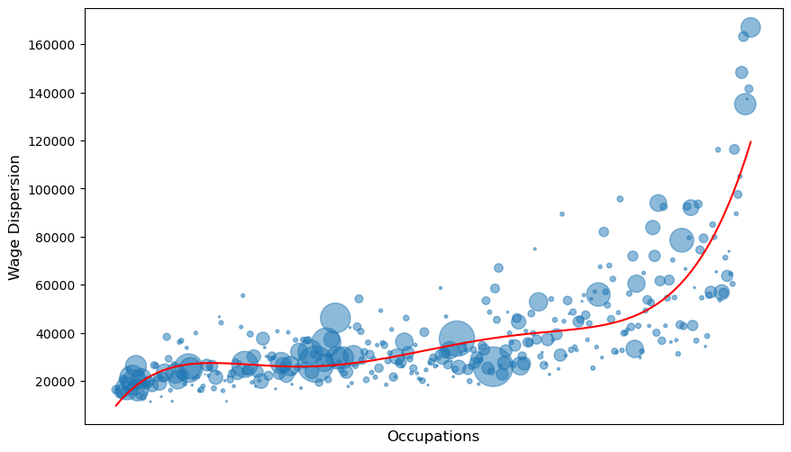
Fig. 16.1 Average wage for each Standard Occupational Classification (SOC) code. The codes are sorted by average wage on the horizontal axis. In red, a polynomial of degree 5 is fitted to the data. The size of the marker is proportional to the number of individuals in the occupation.#
We also plot the average wages for each occupation (SOC code). Again, occupations are ordered by increasing average wage.
# Scatter plot average wage for each occupation
plt.figure(figsize=(10, 6))

# Scatter plot with marker size proportional to count
plt.scatter(
    occupation_df.index,
    occupation_df['mean_Earnings'],
    alpha = 0.5, # transparency
    label = 'Occupations'
)

# Polynomial interpolation
x = np.arange(len(occupation_df))
y = occupation_df['mean_Earnings']
degree = 5
p = np.poly1d(np.polyfit(x, y, degree)  )
plt.plot(x, p(x), color='red')

# Add labels and title
plt.xlabel("Occupations", fontsize=12)
plt.ylabel("Average Wage", fontsize=12)
plt.xticks([], fontsize=8)

plt.show()
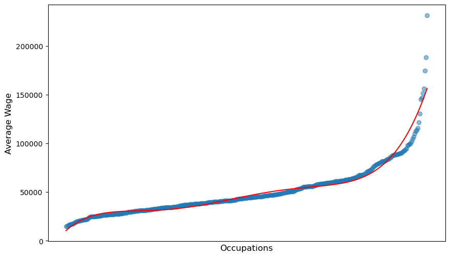
Fig. 16.2 Average wage for each Standard Occupational Classification (SOC) code. The codes are sorted by average wage on the horizontal axis. In red, a polynomial of degree 5 is fitted to the data.#
16.7.2. Model#
parameters_1980 = namedtuple('Params_Jobs', [
    'mean_1', 'var_1', 'mean_2', 'var_2', 'mixing_weight', 'var_workers'
])(
    mean_1=0.38,
    var_1=0.06,
    mean_2=0.0,
    var_2=0.75,
    mixing_weight=0.36,
    var_workers=0.2
)

num_agents=1500
def generate_types_application(self, num_agents, params, random_seed=1):

    mean_1, var_1, mean_2, var_2, mixing_weight, var_workers = params

    np.random.seed(random_seed)

    # Job types
    job_types = np.where(np.random.rand(num_agents) < mixing_weight,
                     np.random.lognormal(mean_1, var_1, num_agents),
                     np.random.lognormal(mean_2, var_2, num_agents))

    # Worker types
    mean_workers = - var_workers/ 2
    worker_types = np.random.lognormal(mean_workers, var_workers, num_agents)

    # Check that worker and job types have distinct values
    assert len(np.unique(worker_types)) == num_agents
    assert len(np.unique(job_types)) == num_agents

    # Assign types to the instance
    self.X_types = worker_types
    self.Y_types = job_types

    # Assign unitary marginals
    self.n_x = np.ones(num_agents, dtype=int)
    self.m_y = np.ones(num_agents, dtype=int)

    # Assign cost matrix
    self.cost_x_y = np.abs(worker_types[:, None] \
                    - job_types[None, :]) ** (1/self.ζ)

ConcaveCostOT.generate_types_application = generate_types_application

# Create an instance of ConcaveCostOT class and generate types
model_1980 = ConcaveCostOT()
model_1980.generate_types_application(num_agents, parameters_1980)
Since we will consider examples with a large number of agents, it will be convenient to visualize the distributions as histograms approximating the pdfs.
def plot_marginals_pdf(self, bins, figsize=(15, 8),
                        range_x_axis=None, title='Distributions of types'):

    plt.figure(figsize=figsize)

    # Plotting histogram for X_types (approximating PDF)
    plt.hist(self.X_types, bins=bins, density=True, color='blue', alpha=0.7,
             label='PDF of worker types',
             edgecolor='blue', range = range_x_axis)

    # Plotting histogram for Y_types (approximating PDF)
    counts, edges = np.histogram(self.Y_types, bins=bins,
                                density=True, range=range_x_axis)
    plt.bar(edges[:-1], -counts, width=np.diff(edges), color='red', alpha=0.7,
            label='PDF of job types ', align='edge', edgecolor='red')

    # Add grid and y=0 axis
    plt.grid(False)
    plt.axhline(0, color='black', linewidth=1)
    plt.gca().spines['bottom'].set_position(('data', 0))

    # Set the x-axis limits based on the range argument
    if range_x_axis is not None:
        plt.xlim(range_x_axis)

    # Labeling the axes and the title
    plt.ylabel('Density')
    plt.title(title)
    plt.gca().yaxis.set_major_locator(MaxNLocator(integer=True))
    plt.legend()
    plt.yticks([])

    plt.show()

ConcaveCostOT.plot_marginals_pdf = plot_marginals_pdf
We plot the histograms and the measure of underqualification for the worker types and job types. We then compute the primal solution and plot the matching.
# Plot pdf
range_x_axis = (0, 4)
model_1980.plot_marginals_pdf(figsize=(8, 5),
                              bins=300, range_x_axis=range_x_axis)
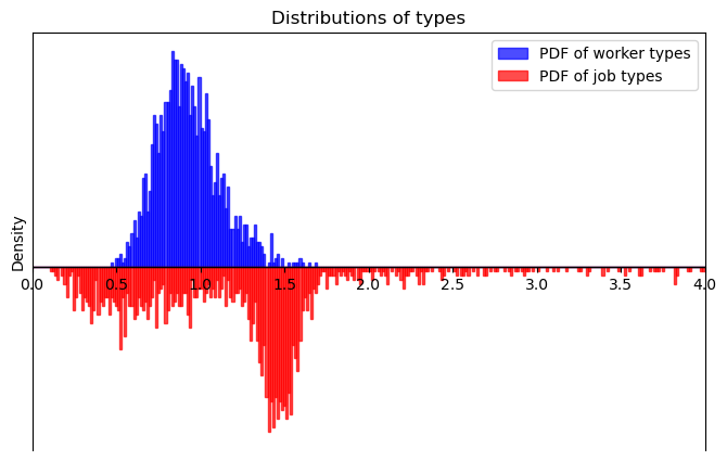
# Plot H_z
model_OD_1980 , _ = model_1980.generate_offD_onD_matching()
model_OD_1980.plot_H_z(figsize=(8, 5), range_x_axis=range_x_axis, scatter=False)
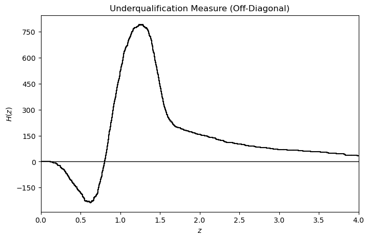
# Compute optimal matching and plot off diagonal matching
matching_1980, matching_OD_1980, model_OD_1980 = model_1980.solve_primal_DSS()
model_OD_1980.plot_matching(matching_OD_1980,
                            title = 'Optimal Matching (off-diagonal)',
                            figsize=(10, 10), plot_H_z=True, scatter=False)
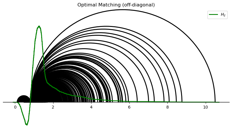
From the optimal matching we compute and visualize the hierarchies.
We then find the dual solution \((\phi,\psi)\) and compute the wages as \(w_x = g(x) - \phi_x,\) assuming that the type-specific productivity of type \(x\) is \(g(x) = x\).
# Find subpairs and plot hierarchies
subpairs, pairs_between = model_OD_1980.find_subpairs(matching_OD_1980,
                                        return_pairs_between=True)
model_OD_1980.plot_hierarchies(subpairs, scatter=False,
                                        range_x_axis=range_x_axis)

# Compute dual solution: φ_x and ψ_y
ϕ_worker_x_1980 , ψ_firm_y_1980 = model_OD_1980.compute_dual_off_diagonal(
                                        subpairs, pairs_between)

# Check dual feasibility
dual_feasibility_i_j = ϕ_worker_x_1980[:,None] + ψ_firm_y_1980[None,:] \
                       - model_OD_1980.cost_x_y
print('Dual feasibility violation:', dual_feasibility_i_j.max())

# Check strong duality
dual_sol = (model_OD_1980.n_x * ϕ_worker_x_1980).sum() \
            + (model_OD_1980.m_y * ψ_firm_y_1980).sum()
primal_sol = (matching_OD_1980 * model_OD_1980.cost_x_y).sum()

print('Value of dual solution: ', dual_sol)
print('Value of primal solution: ', primal_sol)

# Compute wages: wage_x = x - φ_x
wage_worker_x_1980 = model_1980.X_types - ϕ_worker_x_1980
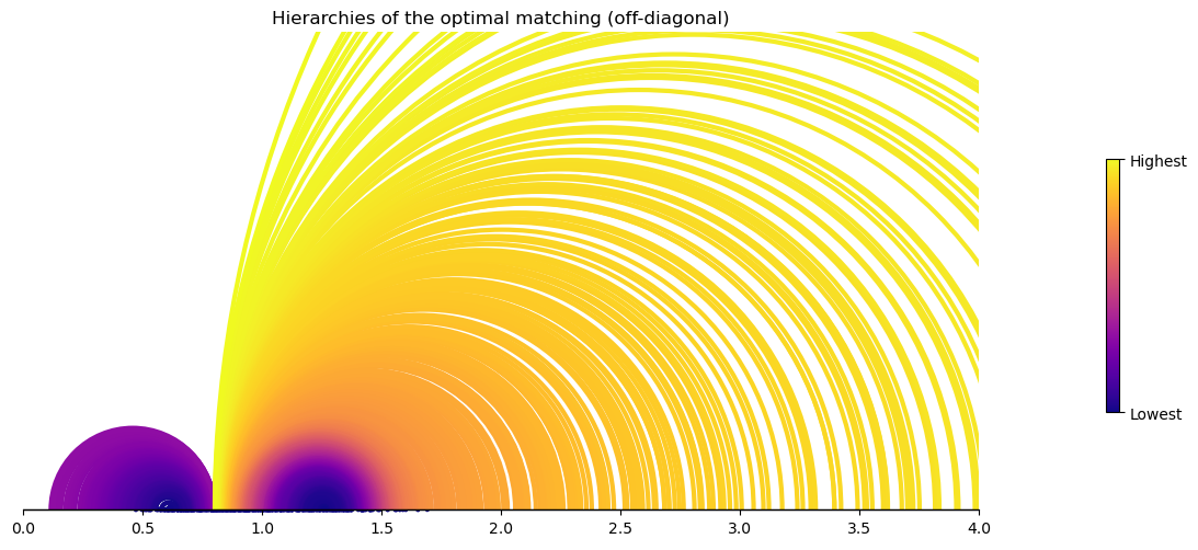
Dual feasibility violation: 4.322138159526534e-08
Value of dual solution:  825.8167029184152
Value of primal solution:  825.8167029184153
Let’s plot average wages and wage dispersion generated by the model.
def plot_wages_application(wages):

    plt.figure(figsize=(10, 6))
    plt.plot(np.sort(wages), label='Wages')
    plt.xlabel("Occupations", fontsize=12)
    plt.ylabel("Wages", fontsize=12)
    plt.grid(True)
    plt.show()


def plot_wage_dispersion_model(wage_worker_x, bins=100,
                                title='Wage Dispersion', figsize=(10, 6)):
    # Compute the percentiles
    percentiles = np.linspace(0, 100, bins + 1)
    bin_edges = np.percentile(wage_worker_x, percentiles)

    # Compute the standard deviation within each percentile range
    stds = []
    for i in range(bins):
        # Compute the standard deviation for the current bin
        bin_data = wage_worker_x[
        (wage_worker_x >= bin_edges[i]) & (wage_worker_x < bin_edges[i + 1])]
        if len(bin_data) > 1:
            stds.append(np.std(bin_data))
        else:
            stds.append(0)

    # Plot the standard deviations for each percentile as bars
    plt.figure(figsize=figsize)
    plt.bar(range(bins), stds, width=1.0, color='grey',
                            alpha=0.7, edgecolor='white')
    plt.xlabel('Percentile', fontsize=12)
    plt.ylabel('Standard Deviation', fontsize=12)
    plt.title(title, fontsize=14)
    plt.grid(axis='y', linestyle='-', alpha=0.6)


plot_wages_application(wage_worker_x_1980)
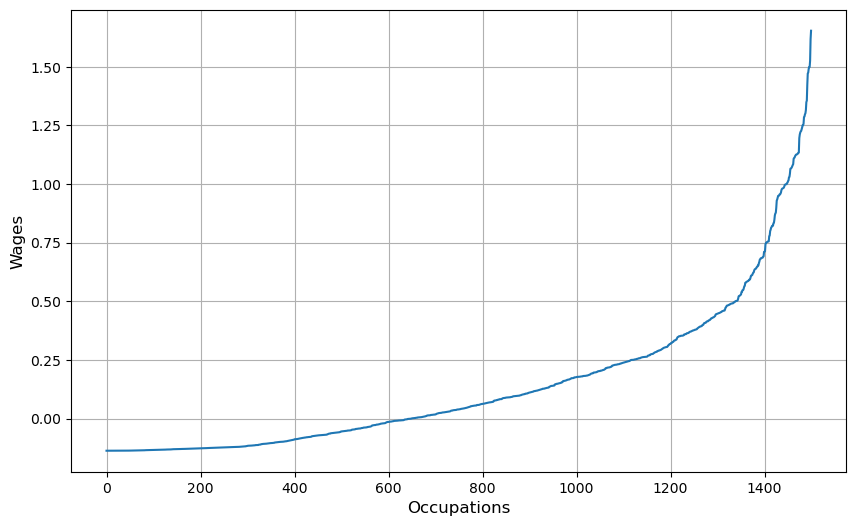
plot_wage_dispersion_model(wage_worker_x_1980, bins=100)
