9. How to Pay for a War: Part 1#

9.1. Overview#

This lecture uses the method of Markov jump linear quadratic dynamic programming that is described in lecture Markov Jump LQ dynamic programming to extend the [Barro, 1979] model of optimal tax-smoothing and government debt in a particular direction.

This lecture has two sequels that offer further extensions of the Barro model

The extensions are modified versions of his 1979 model suggested by [Barro, 1999] and [Barro and McCleary, 2003]).

[Barro, 1979] m is about a government that borrows and lends in order to minimize an intertemporal measure of distortions caused by taxes.

Technical tractability induced [Barro, 1979] to assume that

the government trades only one-period risk-free debt, and
the one-period risk-free interest rate is constant

By using Markov jump linear quadratic dynamic programming we can allow interest rates to move over time in empirically interesting ways.

Also, by expanding the dimension of the state, we can add a maturity composition decision to the government’s problem.

By doing these two things we extend [Barro, 1979] along lines he suggested in [Barro, 1999] and [Barro and McCleary, 2003]).

[Barro, 1979] assumed

that a government faces an exogenous sequence of expenditures that it must finance by a tax collection sequence whose expected present value equals the initial debt it owes plus the expected present value of those expenditures.
that the government wants to minimize a measure of tax distortions that is proportional to \(E_0 \sum_{t=0}^{\infty} \beta^t T_t^2\), where \(T_t\) are total tax collections and \(E_0\) is a mathematical expectation conditioned on time \(0\) information.
that the government trades only one asset, a risk-free one-period bond.
that the gross interest rate on the one-period bond is constant and equal to \(\beta^{-1}\), the reciprocal of the factor \(\beta\) at which the government discounts future tax distortions.

Barro’s model can be mapped into a discounted linear quadratic dynamic programming problem.

Partly inspired by [Barro, 1999] and [Barro and McCleary, 2003], our generalizations of [Barro, 1979], assume

that the government borrows or saves in the form of risk-free bonds of maturities \(1, 2, \ldots , H\).
that interest rates on those bonds are time-varying and in particular, governed by a jointly stationary stochastic process.

Our generalizations are designed to fit within a generalization of an ordinary linear quadratic dynamic programming problem in which matrices that define the quadratic objective function and the state transition function are time-varying and stochastic.

This generalization, known as a Markov jump linear quadratic dynamic program, combines

the computational simplicity of linear quadratic dynamic programming, and
the ability of finite state Markov chains to represent interesting patterns of random variation.

We want the stochastic time variation in the matrices defining the dynamic programming problem to represent variation over time in

interest rates
default rates
roll over risks

As described in Markov Jump LQ dynamic programming, the idea underlying Markov jump linear quadratic dynamic programming is to replace the constant matrices defining a linear quadratic dynamic programming problem with matrices that are fixed functions of an \(N\) state Markov chain.

For infinite horizon problems, this leads to \(N\) interrelated matrix Riccati equations that pin down \(N\) value functions and \(N\) linear decision rules, applying to the \(N\) Markov states.

9.2. Public Finance Questions#

[Barro, 1979] is designed to answer questions such as

Should a government finance an exogenous surge in government expenditures by raising taxes or borrowing?
How does the answer to that first question depend on the exogenous stochastic process for government expenditures, for example, on whether the surge in government expenditures can be expected to be temporary or permanent?

[Barro, 1999] and [Barro and McCleary, 2003] are designed to answer more fine-grained questions such as

What determines whether a government wants to issue short-term or long-term debt?
How do roll-over risks affect that decision?
How does the government’s long-short portfolio management decision depend on features of the exogenous stochastic process for government expenditures?

Thus, both the simple and the more fine-grained versions of Barro’s models are ways of precisely formulating the classic issue of How to pay for a war.

This lecture describes:

An application of Markov jump LQ dynamic programming to a model in which a government faces exogenous time-varying interest rates for issuing one-period risk-free debt.

A sequel to this lecture describes applies Markov LQ control to settings in which a government issues risk-free debt of different maturities.

!pip install --upgrade quantecon

Let’s start with some standard imports:

import quantecon as qe
import numpy as np
import matplotlib.pyplot as plt

9.3. Barro (1979) Model#

We begin by solving a version of [Barro, 1979] by mapping it into the original LQ framework.

As mentioned in this lecture, the Barro model is mathematically isomorphic with the LQ permanent income model.

Let

\(T_t\) denote tax collections
\(\beta\) be a discount factor
\(b_{t,t+1}\) be time \(t+1\) goods that at \(t\) the government promises to deliver to time \(t\) buyers of one-period government bonds
\(G_t\) be government purchases
\(p_{t,t+1}\) the number of time \(t\) goods received per time \(t+1\) goods promised to one-period bond purchasers.

Evidently, \(p_{t, t+1}\) is inversely related to appropriate corresponding gross interest rates on government debt.

In the spirit of [Barro, 1979], the stochastic process of government expenditures is exogenous.

The government’s problem is to choose a plan for taxation and borrowing \(\{b_{t+1}, T_t\}_{t=0}^\infty\) to minimize

\[ E_0 \sum_{t=0}^\infty \beta^t T_t^2 \]

subject to the constraints

\[ T_t + p_{t,t+1} b_{t,t+1} = G_t + b_{t-1,t} \]

\[ G_t = U_{g} z_t \]

\[ z_{t+1} = A_{22} z_t + C_{2} w_{t+1} \]

where \(w_{t+1} \sim {\cal N}(0,I)\)

The variables \(T_t, b_{t, t+1}\) are control variables chosen at \(t\), while \(b_{t-1,t}\) is an endogenous state variable inherited from the past at time \(t\) and \(p_{t,t+1}\) is an exogenous state variable at time \(t\).

To begin, we assume that \(p_{t,t+1}\) is constant (and equal to \(\beta\))

later we will extend the model to allow \(p_{t,t+1}\) to vary over time

To map into the LQ framework, we use \(x_t = \begin{bmatrix} b_{t-1,t} \\ z_t \end{bmatrix}\) as the state vector, and \(u_t = b_{t,t+1}\) as the control variable.

Therefore, the \((A, B, C)\) matrices are defined by the state-transition law:

\[\begin{split} x_{t+1} = \begin{bmatrix} 0 & 0 \\ 0 & A_{22} \end{bmatrix} x_t + \begin{bmatrix} 1 \\ 0 \end{bmatrix} u_t + \begin{bmatrix} 0 \\ C_2 \end{bmatrix} w_{t+1} \end{split}\]

To find the appropriate \((R, Q, W)\) matrices, we note that \(G_t\) and \(b_{t-1,t}\) can be written as appropriately defined functions of the current state:

\[ G_t = S_G x_t \hspace{2mm}, \hspace{2mm} b_{t-1,t} = S_1 x_t \]

If we define \(M_t = - p_{t,t+1}\), and let \(S = S_G + S_1\), then we can write taxation as a function of the states and control using the government’s budget constraint:

\[ T_t = S x_t + M_t u_t \]

It follows that the \((R, Q, W)\) matrices are implicitly defined by:

\[ T_t^2 = x_t'S'Sx_t + u_t'M_t'M_tu_t + 2 u_t'M_t'S x_t \]

If we assume that \(p_{t,t+1} = \beta\), then \(M_t \equiv M = -\beta\).

In this case, none of the LQ matrices are time varying, and we can use the original LQ framework.

We will implement this constant interest-rate version first, assuming that \(G_t\) follows an AR(1) process:

\[ G_{t+1} = \bar G + \rho G_t + \sigma w_{t+1} \]

To do this, we set \(z_t = \begin{bmatrix} 1 \\ G_t \end{bmatrix}\), and consequently:

\[\begin{split} A_{22} = \begin{bmatrix} 1 & 0 \\ \bar G & \rho \end{bmatrix} \hspace{2mm} , \hspace{2mm} C_2 = \begin{bmatrix} 0 \\ \sigma \end{bmatrix} \end{split}\]

# Model parameters
β, Gbar, ρ, σ = 0.95, 5, 0.8, 1

# Basic model matrices
A22 = np.array([[1,    0],
                [Gbar, ρ],])

C2 = np.array([[0],
               [σ]])

Ug = np.array([[0, 1]])

# LQ framework matrices
A_t = np.zeros((1, 3))
A_b = np.hstack((np.zeros((2, 1)), A22))
A = np.vstack((A_t, A_b))

B = np.zeros((3, 1))
B[0, 0] = 1

C = np.vstack((np.zeros((1, 1)), C2))

Sg = np.hstack((np.zeros((1, 1)), Ug))
S1 = np.zeros((1, 3))
S1[0, 0] = 1
S = S1 + Sg

M = np.array([[-β]])

R = S.T @ S
Q = M.T @ M
W = M.T @ S

# Small penalty on the debt required to implement the no-Ponzi scheme
R[0, 0] = R[0, 0] + 1e-9

We can now create an instance of LQ:

LQBarro = qe.LQ(Q, R, A, B, C=C, N=W, beta=β)
P, F, d = LQBarro.stationary_values()
x0 = np.array([[100, 1, 25]])

We can see the isomorphism by noting that consumption is a martingale in the permanent income model and that taxation is a martingale in Barro’s model.

We can check this using the \(F\) matrix of the LQ model.

Because \(u_t = -F x_t\), we have

\[ T_t = S x_t + M u_t = (S - MF) x_t \]

and

\[ T_{t+1} = (S-MF)x_{t+1} = (S-MF)(Ax_t + B u_t + C w_{t+1}) = (S-MF)((A-BF)x_t + C w_{t+1}) \]

Therefore, the mathematical expectation of \(T_{t+1}\) conditional on time \(t\) information is

\[ E_t T_{t+1} = (S-MF)(A-BF)x_t \]

Consequently, taxation is a martingale (\(E_t T_{t+1} = T_t\)) if

\[ (S-MF)(A-BF) = (S-MF) , \]

which holds in this case:

S - M @ F, (S - M @ F) @ (A - B @ F)

(array([[ 0.05000002, 19.79166502,  0.2083334 ]]),
 array([[ 0.05000002, 19.79166504,  0.2083334 ]]))

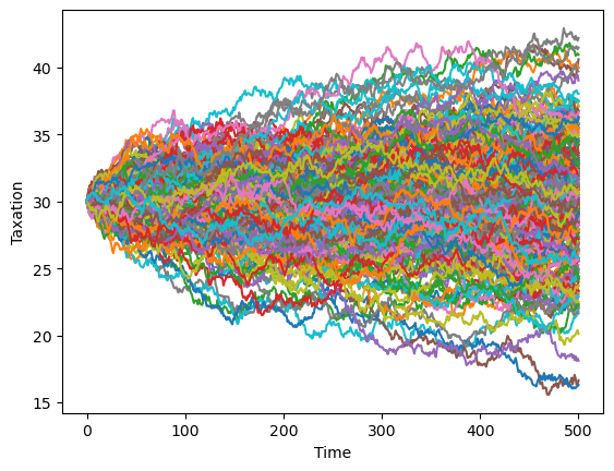
This explains the fanning out of the conditional empirical distribution of taxation across time, computed by simulating the Barro model many times and averaging over simulated paths:

T = 500
for i in range(250):
    x, u, w = LQBarro.compute_sequence(x0, ts_length=T)
    plt.plot(list(range(T+1)), ((S - M @ F) @ x)[0, :])
plt.xlabel('Time')
plt.ylabel('Taxation')
plt.show()

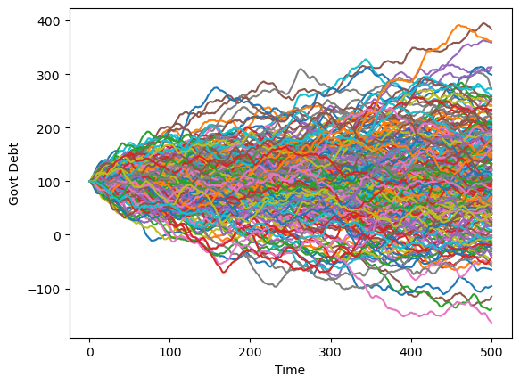
_images/d03f6320fa3fc29adcb3d20c5e92dff14f6a20920948057781863060a6231c61.png

We can see a similar, but a smoother pattern, if we plot government debt over time.

T = 500
for i in range(250):
    x, u, w = LQBarro.compute_sequence(x0, ts_length=T)
    plt.plot(list(range(T+1)), x[0, :])
plt.xlabel('Time')
plt.ylabel('Govt Debt')
plt.show()

_images/75ce5e8e876831fe11b437bf822e95d4982dab9bbfdc084d66fcfbcef59edf55.png

9.4. Python Class to Solve Markov Jump Linear Quadratic Control Problems#

To implement the extension to the Barro model in which \(p_{t,t+1}\) varies over time, we must allow the M matrix to be time-varying.

Our \(Q\) and \(W\) matrices must also vary over time.

We can solve such a model using the LQMarkov class that solves Markov jump linear quandratic control problems as described above.

The code for the class can be viewed here.

The class takes lists of matrices that corresponds to \(N\) Markov states.

The value and policy functions are then found by iterating on a coupled system of matrix Riccati difference equations.

Optimal \(P_s,F_s,d_s\) are stored as attributes.

The class also contains a method that simulates a model.

9.5. Barro Model with a Time-varying Interest Rate#

We can use the above class to implement a version of the Barro model with a time-varying interest rate.

A simple way to extend the model is to allow the interest rate to take two possible values.

We set:

\[ p^1_{t,t+1} = \beta + 0.02 = 0.97 \]

\[ p^2_{t,t+1} = \beta - 0.017 = 0.933 \]

Thus, the first Markov state has a low interest rate and the second Markov state has a high interest rate.

We must also specify a transition matrix for the Markov state.

We use:

\[\begin{split} \Pi = \begin{bmatrix} 0.8 & 0.2 \\ 0.2 & 0.8 \end{bmatrix} \end{split}\]

Here, each Markov state is persistent, and there is are equal chances of moving from one state to the other.

The choice of parameters means that the unconditional expectation of \(p_{t,t+1}\) is 0.9515, higher than \(\beta (=0.95)\).

If we were to set \(p_{t,t+1} = 0.9515\) in the version of the model with a constant interest rate, government debt would explode.

# Create list of matrices that corresponds to each Markov state
Π = np.array([[0.8, 0.2],
              [0.2, 0.8]])

As = [A, A]
Bs = [B, B]
Cs = [C, C]
Rs = [R, R]

M1 = np.array([[-β - 0.02]])
M2 = np.array([[-β + 0.017]])

Q1 = M1.T @ M1
Q2 = M2.T @ M2
Qs = [Q1, Q2]
W1 = M1.T @ S
W2 = M2.T @ S
Ws = [W1, W2]

# create Markov Jump LQ DP problem instance
lqm = qe.LQMarkov(Π, Qs, Rs, As, Bs, Cs=Cs, Ns=Ws, beta=β)
lqm.stationary_values();

The decision rules are now dependent on the Markov state:

lqm.Fs[0]

array([[-0.98437712, 19.20516427, -0.8314215 ]])

lqm.Fs[1]

array([[-1.01434301, 21.5847983 , -0.83851116]])

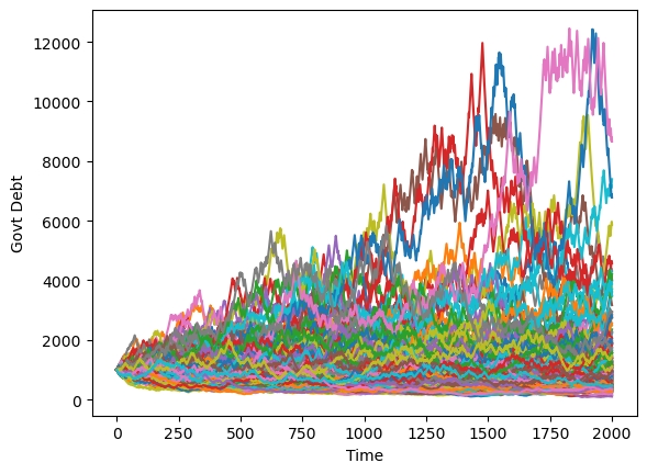
Simulating a large number of such economies over time reveals interesting dynamics.

Debt tends to stay low and stable but recurrently surges.

T = 2000
x0 = np.array([[1000, 1, 25]])
for i in range(250):
    x, u, w, s = lqm.compute_sequence(x0, ts_length=T)
    plt.plot(list(range(T+1)), x[0, :])
plt.xlabel('Time')
plt.ylabel('Govt Debt')
plt.show()

_images/23ef38abc2775b16b23a0f34050fcbd97e52ec505febcd029fe8b34ad1d33959.png