23. Gorman Aggregation#
23.1. Overview#
Gorman [1953] described a class of models with preferences having the useful property that there exists a “representative household” in the sense that competitive equilibrium allocations can be computed in the following way:
take the heterogeneous preferences of a diverse collection of households and from them synthesize the preferences of a single “representative household”
assign the endowments of all households to the representative household
construct a competitive equilibrium allocation and price system for the representative agent economy
at the competitive equilibrium price system, compute the wealth – i.e., the present value – of each household’s initial endowment
find a consumption plan for each household that maximizes its utility functional subject to the wealth that you computed in the previous step
This procedure allows us to compute the competitive equilibrium price system for the heterogeneous household economy prior to computing the competitive equilibrium allocation.
That substantially simplifies calculating a competitive equilibrium.
Note
In general, computing a competitive equilibrium requires solving for the price system and the allocation simultaneously, not recursively.
Chapter 12 of Hansen and Sargent [2013] described how to adapt preference specifications of Gorman [1953] to a linear-quadratic class of environments.
This lecture uses the quantecon.DLE class to study economies that satisfy necessary conditions for Gorman
aggregation of preferences.
To compute a competitive equilibrium, our first step will be to form a representative agent.
After that, we can use some of our DLE tools to compute competitive equilibrium
prices without knowing the allocation of consumption to individual households
households’ individual wealth levels
households’ consumption levels
Thus, this lecture builds on tools and Python code described in Recursive Models of Dynamic Linear Economies, Growth in Dynamic Linear Economies, and IRFs in Hall Models.
In a little more detail, when conditions for Gorman aggregation of preferences are satisfied, we can compute a competitive equilibrium of a heterogeneous-household economy in two steps: solve a representative-agent linear-quadratic planning problem for aggregates, then recover household allocations via a sharing-formula that makes each household’s consumption a household-specific constant share of aggregate consumption.
a household’s share parameter will depend on the implicit Pareto weight implied by the initial distribution of endowment.
The key is that the Gorman-aggregation conditions ensure all households have parallel Engel curves.
That feature is what lets us determine the aggregate allocations and price system before we compute the distribution of the aggregate allocation among individual households.
This eliminates the usual feature that the utility possibility frontier shifts with endowment changes, making it impossible to rank allocations without specifying distributional weights.
Note
Computing a competitive equilibrium typically entails solving a fixed point problem.
Negishi [1960] described a social welfare function that is maximized, subject to resource and technological constraints, by a competitive equilibrium allocation.
For Negishi, that social welfare function is a “linear combination of the individual utility functions of households, with the weights in the combination in inverse proportion to the marginal utilities of income.”
Because Negishi’s weights depend on the allocation through the marginal utilities of income, computing a competitive equilibrium via constrained maximization of a Negishi-style welfare function requires finding a fixed point in the weights.
When they apply, the beauty of Gorman’s aggregation conditions is that time series aggregates and market prices can be computed without resorting to Negishi’s fixed point approach.
With the help of this powerful result, we proceed in two steps:
Solve the planner’s problem and compute selection matrices that map the aggregate state into allocations and prices.
Compute household-specific policies and the Gorman sharing rule.
For a special case described in Section 12.6 of Hansen and Sargent [2013], where preference shocks are inactive, we can also
Implement the Arrow-Debreu allocation by allowing households to trade a risk-free one-period bond and a single mutual fund that owns all of the economy’s physical capital.
We shall provide examples of these steps in economies with two and then with many households.
Before studying these things in the context of the DLE class, we’ll first introduce Gorman aggregation in a static economy.
In addition to what’s in Anaconda, this lecture uses the quantecon library
!pip install --upgrade quantecon
We make the following imports
import numpy as np
from scipy.linalg import solve_discrete_are
from quantecon import DLE
from quantecon import LQ
import matplotlib.pyplot as plt
23.1.1. Gorman aggregation in a static economy#
To indicate where our competitive equilibrium sharing rule originates, we start with a static economy with \(n\) goods, price vector \(p\), and households \(j = 1, \ldots, J\).
Let \(c^a\) denote the aggregate amount of consumption to be allocated among households.
Associated with \(c^a\) is an Edgeworth box and a set of Pareto optimal allocations.
From the Pareto optimal allocations, one can construct utility allocation surfaces that describe the frontier of alternative feasible utility assignments to individual households.
Imagine moving from the aggregate vector \(c^a\) to some other vector \(\tilde{c}^a\) and hence to a new Edgeworth box.
If neither the original box nor the new box contains the other, then it is possible that the utility allocation surfaces for the two boxes may cross, in which case there exists no ordering of aggregate consumption that is independent of the utility weights assigned to individual households.
Here is an example showing when aggregation fails.
Consider a two-person, two-good, pure-exchange economy where agent A has utility function \(U^A = X_A^{1/3} Y_A^{2/3}\), while consumer B has utility function \(U^B = X_B^{2/3} Y_B^{1/3}\).
With aggregate endowment pairs \(E = (8,3)\) and \(E = (3,8)\), the utility possibility frontiers cross, indicating that these two aggregate endowment vectors cannot be ranked in a way that ignores how utility is distributed between consumers A and B.
Furthermore, for a given endowment, the slope of the consumers’ indifference curves at the tangencies that determine the contract curve varies as one moves along the contract curve.
This means that for a given aggregate endowment, the competitive equilibrium price depends on the allocation between consumers A and B.
It follows that for this economy, one cannot determine equilibrium prices independently of the equilibrium allocation.
The crossing of the utility possibility frontiers can be seen by plotting the efficient utility pairs for each aggregate endowment
def frontier(X_total, Y_total, grid_size=500):
    """
    Compute a utility possibility frontier by tracing the contract curve.

    Preferences:
      U^A = X_A^(1/3) Y_A^(2/3)
      U^B = X_B^(2/3) Y_B^(1/3)
    """
    xA = np.linspace(1e-6, X_total - 1e-6, grid_size)
    yA = (4 * xA * Y_total) / (X_total + 3 * xA)  # contract curve
    xB, yB = X_total - xA, Y_total - yA

    UA = (xA ** (1 / 3)) * (yA ** (2 / 3))
    UB = (xB ** (2 / 3)) * (yB ** (1 / 3))
    return UA, UB


UA1, UB1 = frontier(8.0, 3.0)
UA2, UB2 = frontier(3.0, 8.0)

fig, ax = plt.subplots()
ax.plot(UA1, UB1, lw=2, label=r"$E=(8,3)$")
ax.plot(UA2, UB2, lw=2, label=r"$E=(3,8)$")
ax.set_xlabel("utility of agent A")
ax.set_ylabel("utility of agent B")
ax.legend()
plt.show()

Fig. 23.1 utility possibility frontiers cross when aggregation fails#
Gorman [1953] described restrictions on preferences under which it is possible to obtain a community preference ordering.
Whenever Gorman’s conditions are satisfied, there occur substantial simplifications in solving multiple-consumer optimal resource allocation problems: in intertemporal contexts, it becomes possible first to determine the optimal allocation of aggregate resources over time, and then allocate aggregate consumption among consumers by assigning utility levels to each person.
There is flexibility in the choice of monotonic transformations that we can use to represent utility levels.
We restrict the utility index to be either nonnegative or nonpositive.
In both cases, we define consumer-specific baseline indifference curves \(\psi_j(p)\) associated with a utility level of zero.
The functions \(\psi_j\) are gradients of concave functions that are positively homogeneous of degree one.
To represent a common departure for all consumers from their baseline indifference curves, we introduce a function \(\psi_c(p)\).
This lets the compensated demand function for consumer \(j\) be represented as
where \(u^j\) is a scalar utility index for consumer \(j\).
The function \(\psi_c\) is the gradient of a positively homogeneous of degree one function that is concave when the utility indices are restricted to be nonnegative and convex when they are restricted to be nonpositive.
It follows that \(\psi_j\) and \(\psi_c\) are homogeneous of degree zero in prices, which means that the implied indifference curves depend only on ratios of prices to an arbitrarily chosen numeraire.
The baseline indifference curves are either the highest or lowest indifference curves, corresponding respectively to cases in which the utility indices \(u^j\) are restricted to be nonpositive or nonnegative.
As noted by Gorman, when preferences are of this form, there is a well-defined compensated demand function for a fictitious representative agent obtained by aggregating individual demands:
where
In this case, optimal resource allocation in a heterogeneous consumer economy simplifies as follows.
Preferences for aggregate consumption define a community preference ordering.
This preference ordering can be combined with a specification of the technology for producing consumption goods to determine the optimal allocation of aggregate consumption.
The mapping \(c^a = \psi_a(p) + u^a \psi_c(p)\) can be inverted to obtain a gradient vector \(p\) that is independent of how utilities are allocated across consumers.
Since \(\psi_c\) and \(\psi_a\) are homogeneous of degree zero, gradients are determined only up to a scalar multiple.
Armed with \(p\), we can then allocate utility among \(J\) consumers while respecting the adding-up constraint (23.1).
The allocation of aggregate consumption across goods and the associated gradient are determined independently of how aggregate utility is divided among consumers.
A decentralized version of this analysis proceeds as follows.
Let \(W^j\) denote the wealth of consumer \(j\) and \(W^a\) denote aggregate wealth. Then \(W^j\) should satisfy
Solving for \(u^j\) gives
Hence, the Engel curve for consumer \(j\) is
Notice that the coefficient on \(W^j\) is the same for all \(j\) since \(\psi_c(p)/(p \cdot \psi_c(p))\) is a function only of the price vector \(p\).
The individual allocations can be determined from the Engel curves by substituting for \(p\) the gradient vector obtained from the representative agent’s optimal allocation problem.
In the quadratic specifications used in this lecture (and in Hansen and Sargent [2013]), the baseline components are degenerate in the sense that \(\psi_j(p) = \chi^j\) is independent of \(p\), where \(\chi^j\) is a consumer-specific bliss point represented by a vector with the same dimension as \(c^j\).
In that case, the demand functions simplify to
where \(\chi^a = \sum_j \chi^j\).
Solving the aggregate equation for the common term \(\psi_c(p) = (c^a - \chi^a)/u^a\) and substituting into the individual equation gives
which rearranges to the static sharing rule
so that there is a common scale factor \((u^j/u^a)\) across all goods for person \(j\).
Hence the fraction of total utility assigned to consumer \(j\) determines his fraction of the vector \((c^a - \chi^a)\).
This is exactly the form we will see in (23.11) below, except that goods are indexed by both dates and states in subscripts.
In the dynamic setting, we set the utility index \(u^j\) equal to household \(j\)’s time-zero marginal utility of wealth \(\mu_{0j}^w\), the Lagrange multiplier on the intertemporal budget constraint.
The ratio \(\mu_{0j}^w / \mu_{0a}^w\) (where \(\mu_{0a}^w = \sum_j \mu_{0j}^w\)) then serves as the time-invariant Pareto weight that determines household \(j\)’s share of aggregate consumption in excess of baseline.
23.2. Dynamic, Stochastic Economy#
We now introduce our basic setup for our dynamic heterogeneous-household economy.
Time is discrete, \(t = 0,1,2,\dots\).
All households share a common discount factor \(\beta \in (0,1)\).
Households are indexed by \(j = 1, \ldots, J\), where \(J\) denotes the total number of households in the economy.
23.2.1. Exogenous state#
The exogenous state \(z_t\) follows a first-order vector autoregression
where \(A_{22}\) governs persistence and \(C_2\) maps i.i.d. shocks \(w_{t+1}\) into the state.
Here we take \(\mathbb{E}[w_{t+1}] = 0\) and \(\mathbb{E}[w_{t+1} w_{t+1}^\top] = I\).
The vector \(z_t\) typically contains three types of components.
Constant: The first element is set to 1 and remains constant.
Aggregate shocks: Components with persistent dynamics that affect all households.
In Example: two-household economy, an AR(2) process drives aggregate endowment fluctuations.
Idiosyncratic shocks: Components that enter individual endowments with loadings summing to zero across households.
These generate cross-sectional heterogeneity while preserving aggregate resource constraints.
The selection matrices \(U_b\) and \(U_d\) pick out which components of \(z_t\) affect household preferences (bliss points) and endowments.
This structure allows us to model both aggregate and idiosyncratic shocks within a unified framework at a later stage.
23.2.2. Technologies#
The economy’s resource constraint is
and
Here \(h_t\) is the aggregate household service, \(s_t\) is the aggregate service flow derived from household capital, \(c_t\) is aggregate consumption, \(i_t\) is investment, \(k_t\) is the aggregate physical capital stock, \(d_t\) is the aggregate endowment (or dividend) stream, and \(g_t\) is the aggregate “intermediate good” (interpreted as total labor supply in this lecture).
The matrices \(\Phi_c, \Phi_g, \Phi_i\) and \(\Gamma\) allow for multiple goods and a general linear mapping from stocks and endowments into resources.
In the one-good case used in the limited-markets section, these reduce to scalars and the resource constraint becomes \(c_t + i_t = \gamma_1 k_{t-1} + d_t\).
We write \(\Pi_h\) for the household service-technology matrix \(\Pi\) in Hansen and Sargent [2013].
23.2.3. The individual household problem#
Recall that we operate in an economy with \(J\) households indexed by \(j = 1, 2, \ldots, J\).
Households differ in preferences and endowments but share a common information set.
Household \(j\) maximizes
subject to the household service technology
and the intertemporal budget constraint
where \(b_{jt} = U_b^j z_t\) is household \(j\)’s preference shock, \(d_{jt} = U_d^j z_t\) is household \(j\)’s endowment stream, \(h_{j,-1}\) and \(k_{j,-1}\) are given initial capital stocks, and \(\ell_{jt}\) is household labor supply.
Here \(\mathbb{E}_0\) is expectation conditional on time-zero information \(\mathcal{J}_0\).
The prices are:
\(p_{0t}\): the time-0 Arrow-Debreu price vector for date-\(t\) consumption goods (across states), so \(p_{0t} \cdot c_{jt}\) is the time-0 value of date-\(t\) consumption
\(w_{0t}\): the time-0 value of date-\(t\) labor
\(\alpha_{0t}\): the time-0 price vector for date-\(t\) endowments (dividends)
\(v_0\): the time-0 value of initial capital
These prices are determined in equilibrium.
In the DLE implementation below, these time-0 prices are recovered from the aggregate solution and encoded in the pricing objects M_c, M_d, M_g, and M_k.
This specification confines heterogeneity among households to four sources:
Differences in the preference processes \(\{b_{jt}\}\), represented by different selections of \(U_b^j\).
Differences in the endowment processes \(\{d_{jt}\}\), represented by different selections of \(U_d^j\).
Differences in initial household capital \(h_{j,-1}\).
Differences in initial physical capital \(k_{j,-1}\).
The matrices \(\Lambda, \Pi_h, \Delta_h, \Theta_h\) do not depend on \(j\).
Because the technology matrices are common across households, every household’s demand system has the same functional form.
All households observe the same aggregate information set \(\{\mathcal{J}_t\}\); in our Markov setting we can take \(\mathcal{J}_t\) to be generated by the current aggregate state \(x_t\).
These restrictions enable Gorman aggregation by ensuring that household demands are affine in wealth.
This will allow us to solve for aggregate allocations and prices without knowing the distribution of wealth across households, as we shall see in Consumption sharing rules.
23.2.4. The representative agent problem#
We construct aggregates by summing across households:
Aggregates are economy-wide totals: \(c_t := \sum_j c_{jt}\), \(b_t := \sum_j b_{jt}\), \(d_t := \sum_j d_{jt}\), and similarly for \((i_t, k_t, h_t, s_t, g_t)\).
Under the Gorman/LQ restrictions, we can compute equilibrium prices and aggregate quantities by synthesizing a fictitious representative agent whose first-order conditions generate equations that determine correct equilibrium prices and a correct aggregate consumption allocation and aggregate capital process.
these equations will not be sufficient to determine the allocation of aggregate consumption among individual households.
Posing a social planning problem for a representative agent is thus a device for computing the correct aggregate allocation along with correct competitive equilibrium prices.
The social planner in our representative agent economy maximizes
subject to the technology constraints (23.3) and (23.4), and the exogenous state process (23.2).
The variable \(g_t\) is the aggregate intermediate good.
With quadratic labor costs and linear budget terms, household \(j\)’s intratemporal first-order condition implies \(\ell_{jt} = \mu^w_{0j} w_{0t}\), where \(\mu^w_{0j}\) is household \(j\)’s time-zero marginal utility of wealth.
Aggregating gives \(g_t := \sum_j \ell_{jt} = \mu^w_{0a} w_{0t}\), where \(\mu^w_{0a}=\sum_j \mu^w_{0j}\).
Hence, the representative agent is constructed so that its first-order condition delivers the same aggregate relation \(g_t=\mu^w_{0a} w_{0t}\).
Note that constraints above involve lagged stocks \((h_{t-1}, k_{t-1})\) and the current exogenous state \(z_t\).
These predetermined variables form the planner’s state:
The solution expresses each aggregate quantity as a linear function of the state via selection matrices:
Similarly, shadow prices are linear in \(x_t\):
These shadow prices correspond to competitive equilibrium prices.
23.2.5. Consumption sharing rules#
This section presents the Gorman consumption sharing rules.
Our preference specification is an infinite-dimensional generalization of the static Gorman setup described in Gorman aggregation in a static economy, where goods are indexed by both dates and states of the world.
Let \(\mu_{0j}^w\) denote household \(j\)’s time-zero marginal utility of wealth, the Lagrange multiplier on its intertemporal budget constraint.
Define the aggregate multiplier as
The ratio \(\mu_{0j}^w / \mu_{0a}^w\) is time-invariant and depends only on information available at time zero.
For convenience, we write
so that \(\sum_j \mu_j = 1\).
This is household \(j\)’s Pareto weight.
The allocation rule for consumption has the form
or equivalently,
Here \(\mu_j c_t\) is household \(j\)’s proportional share of aggregate consumption and \(\tilde{\chi}_{jt}\) is the deviation from this proportional share.
These deviations sum to zero: \(\sum_j \tilde{\chi}_{jt} = 0\).
The baseline term \(\chi_{jt}\) is determined by the preference shock process \(\{b_{jt}\}\) and initial household capital \(h_{j,-1}\).
We write the aggregate baseline as \(\chi_t := \sum_{j=1}^J \chi_{jt}\).
The beauty of this representation is that the weight \(\mu_j\) is time-invariant.
Nonseparabilities in preferences (over time or across goods) affect only the construction of the baseline process \(\{\chi_{jt}\}\) and the calculation of the weight \(\mu_j\) implied by the distribution of wealth.
23.2.5.1. Household services allocation rule#
First-order necessary conditions for consumption services imply
where \(\rho_{0t}\) is the time-0 shadow price for date-\(t\) services from the aggregate problem.
Since the aggregate first-order condition is \(s_t - b_t = \mu_{0a}^w \rho_{0t}\), we can eliminate \(\rho_{0t}\) to obtain:
or equivalently \(\tilde{s}_{jt} = \tilde{b}_{jt}\), where \(\tilde{y}_{jt} := y_{jt} - \mu_j y_t\) for any variable \(y\).
This representation does not involve prices directly.
23.2.5.2. Inverse canonical representation#
Given \(\rho_{0t}\) from the aggregate solution, we can solve (23.12) for \(s_{jt}\), then use the inverse canonical representation from Chapter 9 of Hansen and Sargent [2013] to compute \(c_{jt}\) and \(h_{jt}\):
with \(h_{j,-1}\) given.
This recursion requires a canonical household technology with square, invertible \(\Pi_h\).
23.2.5.3. Computational details#
Define deviation processes \(\tilde{y}_{jt} := y_{jt} - \mu_j y_t\) for any variable \(y\).
In particular, the deviation durable stock is \(\tilde{h}_{jt} := h_{jt} - \mu_j h_t\).
The deviation form of the inverse canonical representation (23.14) is
with \(\tilde{h}_{j,-1} = h_{j,-1} - \mu_j h_{-1}\) given.
Associated with \(\tilde{s}_{jt}\) is a synthetic consumption process \(\tilde{\chi}_{jt}\) that makes \(\tilde{c}_{jt} = \tilde{\chi}_{jt}\) be the optimal sharing rule.
To construct \(\tilde{\chi}_{jt}\), we substitute \(\tilde{s}_{jt} = \tilde{b}_{jt}\) into the inverse canonical representation:
with \(\tilde{\eta}_{j,-1} = \tilde{h}_{j,-1}\).
Since \(\tilde{s}_{jt} = \tilde{b}_{jt}\) and \(\tilde{\eta}_{j,-1} = \tilde{h}_{j,-1}\), it follows from (23.15) and (23.16) that \(\tilde{c}_{jt} = \tilde{\chi}_{jt}\).
Since the allocation rule for consumption can be expressed as
we can append the recursion for \(c_t\) from the aggregate problem to obtain a recursion generating \(c_{jt}\).
23.2.5.4. Labor allocation rule#
Once the aggregate allocation and prices are obtained from the representative problem, individual labor allocations follow from the ratio of individual to aggregate marginal utilities of wealth:
where \(g_t\) is the aggregate intermediate good determined by the representative agent’s first-order condition.
This step recovers household labor supplies consistent with the competitive equilibrium.
23.2.5.5. Risk sharing#
Because the coefficient \(\mu_j\) is invariant over time and across goods, allocation rule (23.10) implies a form of risk pooling in the deviation process \(\{c_{jt} - \chi_{jt}\}\).
In the special case where the preference shock processes \(\{b_{jt}\}\) are deterministic (in the sense that they reside in the information set \(\mathcal{J}_0\)), individual consumption goods will be perfectly correlated with their aggregate counterparts.
23.3. Household allocations#
A direct way to compute allocations to individuals would be to solve the problem each household faces in competitive equilibrium at equilibrium prices.
For a fixed Lagrange multiplier \(\mu_{0j}^w\) on the household’s budget constraint, the household’s problem can be expressed as an optimal linear regulator with a state vector augmented to reflect aggregate state variables determining scaled Arrow-Debreu prices.
One could compute individual allocations by iterating to find the multiplier \(\mu_{0j}^w\) that satisfies the budget constraint.
But there is a more elegant approach that uses the Gorman allocation rules.
23.3.1. Computing household allocations#
We apply our consumption sharing rules (23.11) and (23.10) in two steps.
23.3.1.1. Step 1: compute deviation consumption#
Using the inverse canonical representation (23.16), we compute the deviation consumption process \(\{\tilde{\chi}_{jt}\}\) from household \(j\)’s deviation bliss points \(\{\tilde{b}_{jt}\}\) and initial deviation state \(\tilde{\eta}_{j,-1} = h_{j,-1} - \mu_j h_{-1}\).
When preferences include durables or habits (\(\Lambda \neq 0\)), the deviation consumption depends on the lagged deviation state \(\tilde{\eta}_{j,t-1}\).
The code solves this as a linear-quadratic control problem using a scaling trick: multiplying the transition matrices by \(\sqrt{\beta}\) converts the discounted problem into an undiscounted one that can be solved with a standard discrete algebraic Riccati equation.
23.3.1.2. Step 2: compute each Pareto weight#
We compute the Pareto weight \(\mu_j\) from household \(j\)’s budget constraint.
We compute five present values:
\(W_d\): present value of household \(j\)’s endowment stream \(\{d_{jt}\}\)
\(W_k\): value of household \(j\)’s initial capital \(k_{j,-1}\)
\(W_{c1}\): present value of the “unit” consumption stream (what it costs to consume \(c_t\))
\(W_{c2}\): present value of the deviation consumption stream \(\{\tilde{\chi}_{jt}\}\)
\(W_g\): present value of the intermediate good stream \(\{g_t\}\)
Formally, (suppressing state indices inside the dot products),
We compute each present value by using doublej2 to sum infinite series.
The budget constraint (23.7) requires that the present value of consumption equals wealth:
From the Gorman allocation rule \(\ell_{jt} = \mu_j g_t\), the present value of labor income is
Substituting the sharing rule \(c_{jt} = \mu_j c_t + \tilde{\chi}_{jt}\) into the left side gives
Solving for \(\mu_j\):
The numerator is household \(j\)’s wealth – i.e., initial capital plus present value of endowments minus the cost of the deviation consumption stream.
The denominator is the net cost of consuming one unit of aggregate consumption, i.e., the value of consumption minus the value of the intermediate good supplied.
Finally, the code constructs selection matrices \(S_{ci}, S_{hi}, S_{si}\) that map the augmented state \(X_t = [h_{j,t-1}^\top, x_t^\top]^\top\) into household \(j\)’s allocations:
Because the deviation term \(\tilde{\chi}_{jt}\) depends on it through the inverse canonical representation, the augmented state includes household \(j\)’s own lagged durable stock \(h_{j,t-1}\).
def doublej2(A1, B1, A2, B2, tol=1e-15, max_iter=10_000):
    """Compute V = sum_{t=0}^inf A1^t B1 B2' (A2')^t via a doubling algorithm."""
    A1 = np.asarray(A1, dtype=float)
    A2 = np.asarray(A2, dtype=float)
    B1 = np.asarray(B1, dtype=float)
    B2 = np.asarray(B2, dtype=float)

    α1, α2 = A1.copy(), A2.copy()
    V = B1 @ B2.T
    diff, it = np.inf, 0

    while diff > tol and it < max_iter:
        α1_next = α1 @ α1
        α2_next = α2 @ α2
        V_next = V + α1 @ V @ α2.T

        diff = np.max(np.abs(V_next - V))
        α1, α2, V = α1_next, α2_next, V_next
        it += 1

    return V

def heter(
    Λ, Θ_h, Δ_h, Π_h, β,
    Θ_k, Δ_k, A_22, C_2,
    U_bi, U_di,
    A0, C, M_d, M_g, M_k, Γ, M_c,
    x0, h0i, k0i,
    S_h, S_k, S_i, S_g, S_d, S_b, S_c, S_s,
    M_h, M_s, M_i,
    tol=1e-15,
):
    """
    Compute household i selection matrices, the Pareto weight μ_i,
    and valuation objects.
    """
    # Dimensions
    n_s, n_h = np.asarray(Λ).shape
    _, n_c = np.asarray(Θ_h).shape
    n_z, n_w = np.asarray(C_2).shape
    n_k, _ = np.asarray(Θ_k).shape
    n_d, _ = np.asarray(U_di).shape
    n_x = n_h + n_k + n_z

    β = float(np.asarray(β).squeeze())

    ## Household deviation problem

    # scaling trick in Chapter 3 of Hansen and Sargent (2013)
    A = np.asarray(Δ_h, dtype=float) * np.sqrt(β)
    B = np.asarray(Θ_h, dtype=float) * np.sqrt(β)

    Λ = np.asarray(Λ, dtype=float)
    Π_h = np.asarray(Π_h, dtype=float)
    U_bi = np.asarray(U_bi, dtype=float)

    R_hh = Λ.T @ Λ + tol * np.eye(n_h)
    Q_hh = Π_h.T @ Π_h
    S_hh = Π_h.T @ Λ

    if np.linalg.matrix_rank(Q_hh) < max(Q_hh.shape):
        raise ValueError("The Π_h'Π_h block is singular.")

    Q_inv = np.linalg.inv(Q_hh)

    # Eliminate cross term
    A = A - B @ Q_inv @ S_hh
    R_hh = R_hh - S_hh.T @ Q_inv @ S_hh

    V11 = solve_discrete_are(A, B, R_hh, Q_hh)
    Λ_s = np.linalg.solve(Q_hh + B.T @ V11 @ B, B.T @ V11 @ A)

    A0_dev = A - B @ Λ_s
    Λ_s = Λ_s + Q_inv @ S_hh

    # Feedforward for U_bi z_t
    A12 = -B @ Q_inv @ Π_h.T @ U_bi
    R12 = Λ.T @ U_bi - Λ.T @ Π_h @ Q_inv @ Π_h.T @ U_bi + A0_dev.T @ V11 @ A12

    V12 = doublej2(A0_dev.T, R12, A_22, np.eye(n_z))
    Q_opt = np.linalg.inv(Q_hh + B.T @ V11 @ B)
    U_b_s = Q_opt @ B.T @ (V12 @ A_22 + V11 @ A12) + Q_inv @ Π_h.T @ U_bi

    # Undo sqrt β scaling
    A0_dev = A0_dev / np.sqrt(β)

    # Long-run covariance under aggregate law of motion
    V_mat = doublej2(β * A0, C, A0, C) * β / (1 - β)

    # Present value of household endowment stream
    U_di = np.asarray(U_di, dtype=float)
    S_di = np.hstack((np.zeros((n_d, n_h + n_k)), U_di))
    W_d = doublej2(β * A0.T, M_d.T, A0.T, S_di.T)
    W_d = x0.T @ W_d @ x0 + np.trace(M_d @ V_mat @ S_di.T)

    # Present value of intermediate good
    W_g = doublej2(β * A0.T, M_g.T, A0.T, S_g.T)
    W_g = x0.T @ W_g @ x0 + np.trace(M_g @ V_mat @ S_g.T)

    # Shadow price object for durables
    M_hs = β * doublej2(β * A0_dev.T, Λ_s.T, A0.T, M_c.T) @ A0
    S_c1 = Θ_h.T @ M_hs - M_c

    # Augmented system for consumption valuation
    A_s = np.block([[A0_dev, Θ_h @ S_c1], [np.zeros((n_x, n_h)), A0]])
    C_s = np.vstack((np.zeros((n_h, n_w)), C))

    M_cs = np.hstack((np.zeros((M_c.shape[0], n_h)), M_c))
    S_cs = np.hstack((-Λ_s, S_c1))

    x0s = np.vstack((np.zeros((n_h, 1)), x0))

    W_c1 = doublej2(β * A_s.T, M_cs.T, A_s.T, S_cs.T)
    V_s = doublej2(β * A_s, C_s, A_s, C_s) * β / (1 - β)
    W_c1 = float(
        (x0s.T @ W_c1 @ x0s + np.trace(M_cs @ V_s @ S_cs.T)).squeeze())

    S_c2 = np.hstack((np.zeros((M_c.shape[0], n_h + n_k)), U_b_s))
    A_s2 = np.block([[A0_dev, Θ_h @ S_c2], [np.zeros((n_x, n_h)), A0]])
    S_cs2 = np.hstack((-Λ_s, S_c2))
    x0s2 = np.vstack((h0i, x0))

    W_c2 = doublej2(β * A_s2.T, M_cs.T, A_s2.T, S_cs2.T)
    V_s2 = doublej2(β * A_s2, C_s, A_s2, C_s) * β / (1 - β)
    W_c2 = float(
        (x0s2.T @ W_c2 @ x0s2 + np.trace(M_cs @ V_s2 @ S_cs2.T)).squeeze())

    # Present value of initial capital
    W_k = float((k0i.T @ (
        np.asarray(Δ_k).T @ M_k +
        np.asarray(Γ).T @ M_d) @ x0).squeeze())

    ## Compute the Pareto weight
    μ = float(((W_k + W_d - W_c2) / (W_c1 - W_g)).squeeze())

    # Household selection matrices on augmented state X_t = [h^i_{t-1}, x_t]
    S_cs = μ * S_c1 + S_c2
    A0_i = np.block([[A0_dev, Θ_h @ S_cs], [np.zeros((n_x, n_h)), A0]])
    S_ci = np.hstack((-Λ_s, S_cs))
    S_hi = A0_i[:n_h, :n_h + n_x]
    S_si = np.hstack((Λ, np.zeros((n_s, n_x)))) + Π_h @ S_ci
    S_bi = np.hstack((np.zeros((n_s, 2 * n_h + n_k)), U_bi))
    S_di = np.hstack((np.zeros((n_d, 2 * n_h + n_k)), U_di))

    # Embed aggregate selection and pricing objects on X_t
    S_ha = np.hstack((np.zeros((n_h, n_h)), S_h))
    S_ka = np.hstack((np.zeros((n_k, n_h)), S_k))
    S_ia = np.hstack((np.zeros((S_i.shape[0], n_h)), S_i))
    S_ga = np.hstack((np.zeros((S_g.shape[0], n_h)), S_g))
    S_da = np.hstack((np.zeros((n_d, n_h)), S_d))
    S_ba = np.hstack((np.zeros((n_s, n_h)), S_b))
    S_ca = np.hstack((np.zeros((S_c.shape[0], n_h)), S_c))
    S_sa = np.hstack((np.zeros((n_s, n_h)), S_s))

    M_ha = np.hstack((np.zeros((M_h.shape[0], n_h)), M_h))
    M_ka = np.hstack((np.zeros((M_k.shape[0], n_h)), M_k))
    M_sa = np.hstack((np.zeros((M_s.shape[0], n_h)), M_s))
    M_ga = np.hstack((np.zeros((M_g.shape[0], n_h)), M_g))
    M_ia = np.hstack((np.zeros((M_i.shape[0], n_h)), M_i))
    M_da = np.hstack((np.zeros((M_d.shape[0], n_h)), M_d))
    M_ca = M_cs

    return {
        "μ": μ,
        "S_ci": S_ci,
        "S_hi": S_hi,
        "S_si": S_si,
        "S_bi": S_bi,
        "S_di": S_di,
        "S_ha": S_ha,
        "S_ka": S_ka,
        "S_ia": S_ia,
        "S_ga": S_ga,
        "S_da": S_da,
        "S_ba": S_ba,
        "S_ca": S_ca,
        "S_sa": S_sa,
        "M_ha": M_ha,
        "M_ka": M_ka,
        "M_sa": M_sa,
        "M_ga": M_ga,
        "M_ia": M_ia,
        "M_da": M_da,
        "M_ca": M_ca,
        "A0_i": A0_i,
        "C_s": C_s,
        "x0s": np.vstack((h0i, x0)),
    }
23.4. Limited markets#
This section studies a special case from Section 12.6 of Hansen and Sargent [2013] in which the Arrow-Debreu allocation can be implemented by opening competitive markets only in a mutual fund and a one-period bond.
So in our setting, we don’t literally require that markets in a complete set of contingent claims be present.
To match the implementation result in Chapter 12.6 of Hansen and Sargent [2013], we specialize to the one-good, constant-return case
In this case, the one-period riskless gross return is constant, \(R = \gamma_1 + \delta_k = 1/\beta\).
We also impose the Chapter 12.6 Hansen and Sargent [2013] measurability restriction that the deviation baseline \(\{\tilde{\chi}_{jt}\}\) is \(\mathcal{J}_0\)-measurable (for example, the preference-shock processes \(\{b_{jt}\}\) are deterministic).
23.4.1. The trading arrangement#
Consider again an economy where each household \(j\) initially owns claims to its own endowment stream \(\{d_{jt}\}\).
Instead of trading in a complete set of Arrow-Debreu markets, we open:
A stock market with securities paying dividends \(\{d_{jt}\}\) for each endowment process
A market for one-period riskless bonds
At time zero, household \(j\) executes the following trades:
Household \(j\) sells all shares of its own endowment security.
Household \(j\) purchases \(\mu_j\) shares of all securities (equivalently, \(\mu_j\) shares of a mutual fund holding the aggregate endowment).
Household \(j\) takes position \(\hat{k}_{j0}\) in the one-period bond.
After this initial rebalancing, household \(j\) maintains a constant risky portfolio share \(\mu_j\) forever, while using the one-period bond for dynamic rebalancing.
The bond position \(\hat{k}_{jt}\) evolves each period according to the recursion derived below.
The portfolio weight \(\mu_j\) is not arbitrary: it is the unique weight that allows the limited-markets portfolio to replicate the Arrow-Debreu consumption allocation.
With Gorman aggregation, household \(j\)’s equilibrium consumption satisfies
We need a portfolio strategy that delivers exactly this consumption stream.
The mutual fund holds claims to all individual endowment streams.
Total dividends paid by the fund each period are
which is the aggregate endowment.
If household \(j\) holds fraction \(\mu_j\) of this fund, it receives \(\mu_j d_t\) in dividends.
The proportional part of consumption \(\mu_j c_t\) must be financed by the mutual fund and by holding a proportional share of aggregate capital.
Combining the resource constraint and capital accumulation gives
Multiplying by \(\mu_j\) yields
so mutual-fund dividends \(\mu_j d_t\) and the return on a proportional capital position \(\mu_j k_{t-1}\) finance household \(j\)’s proportional claim \(\mu_j c_t\) plus the reinvestment needed to maintain its share \(\mu_j k_t\).
The remaining term \(\tilde{\chi}_{jt}\) is financed by adjusting an additional bond position \(\hat{k}_{jt}\) according to the recursion derived below.
Holding \(\mu_j\) shares of the mutual fund thus finances exactly the proportional component \(\mu_j c_t\) (together with rolling over the proportional capital position), while the bond handles the deviation \(\tilde{\chi}_{jt}\).
This transforms heterogeneous endowment risk into proportional shares of aggregate risk.
We now derive the law of motion for the bond position \(\hat{k}_{jt}\).
First, write the budget constraint.
Household \(j\)’s time-\(t\) resources are its mutual fund dividend \(\mu_j d_t\) plus the return on its bond position \(R(\mu_j k_{t-1} + \hat{k}_{j,t-1})\).
Its uses of funds are consumption \(c_{jt}\) plus the new bond position \((\mu_j k_t + \hat{k}_{jt})\), so
Substituting the sharing rule by replacing \(c_{jt}\) with \(\mu_j c_t + \tilde{\chi}_{jt}\) gives:
Using \(\mu_j c_t + \mu_j k_t = R(\mu_j k_{t-1}) + \mu_j d_t\), the proportional terms cancel and we obtain
Rearranging gives the bond recursion:
Equation (23.19) says that the bond position grows at rate \(R\) but is drawn down by the deviation consumption \(\tilde{\chi}_{jt}\).
When \(\tilde{\chi}_{jt} > 0\) (i.e., household \(j\) consumes more than its share), it finances this by running down its bond holdings.
The household’s total asset position is hence \(a_{jt} = \mu_j k_t + \hat{k}_{jt}\).
23.4.2. Initial bond position#
To find \(\hat{k}_{j0}\), we solve the recursion (23.19) forward.
Iterating forward from \(\hat{k}_{jt} = R \hat{k}_{j,t-1} - \tilde{\chi}_{jt}\), we get:
For the budget constraint to hold with equality, we apply transversality and require \(\lim_{T \to \infty} R^{-T} \hat{k}_{jT} = 0\).
Dividing by \(R^T\):
Taking \(T \to \infty\) and using transversality:
Solving for the initial position gives:
This is the present value of future deviation consumption.
Under the measurability restriction (\(\tilde{\chi}_{jt} \in \mathcal{J}_0\)), this sum is known at date zero and can be used to set the initial bond position.
Note
This construction embodies a multiperiod counterpart to an aggregation result for security markets derived by Rubinstein [1974].
In a two-period model, Rubinstein provided sufficient conditions on preferences of households and asset market payoffs that implement a complete-markets Arrow-Debreu contingent claims allocation with incomplete security markets.
In Rubinstein’s implementation, all households hold the same portfolio of risky assets.
In our construction, households also hold the same portfolio of risky assets, and portfolio weights do not vary over time.
All changes over time in portfolio composition take place through transactions in the bond market.
The code below computes household allocations and limited-markets portfolios according to the market structure we have just described.
def compute_household_paths(
            econ, U_b_list, U_d_list, x0, x_path,
            γ_1, Λ, h0i=None, k0i=None):
    """
    Compute household allocations and limited-markets portfolios
    along a fixed aggregate path.
    """

    # Organize inputs
    x0 = np.asarray(x0, dtype=float).reshape(-1, 1)
    x_path = np.asarray(x_path, dtype=float)

    Θ_h = np.atleast_2d(econ.thetah)
    Δ_h = np.atleast_2d(econ.deltah)
    Π_h = np.atleast_2d(econ.pih)
    Λ = np.atleast_2d(Λ)

    n_h = Θ_h.shape[0]
    n_k = np.atleast_2d(econ.thetak).shape[0]

    z_path = x_path[n_h + n_k:, :]


    # Select consumption, capital, bonds, and dividends
    c = econ.Sc @ x_path
    k = econ.Sk @ x_path
    b = econ.Sb @ x_path
    d = econ.Sd @ x_path

    δ_k = float(np.asarray(econ.deltak).squeeze())
    R = δ_k + float(γ_1)

    Π_inv = np.linalg.inv(Π_h)
    A_h = Δ_h - Θ_h @ Π_inv @ Λ
    B_h = Θ_h @ Π_inv

    if h0i is None:
        h0i = np.zeros((n_h, 1))
    if k0i is None:
        k0i = np.zeros((n_k, 1))

    # Prepare data containers
    N = len(U_b_list)
    _, T = c.shape

    μ = np.empty(N)
    χ_tilde = np.zeros((N, T))
    c_j = np.zeros((N, T))
    d_j = np.zeros((N, T))
    d_share = np.zeros((N, T))  # Dividend income under limited markets
    k_share = np.zeros((N, T))
    k_hat = np.zeros((N, T))
    a_total = np.zeros((N, T))

    # For each household, compute Pareto weight and paths
    for j in range(N):
        U_bj = np.asarray(U_b_list[j], dtype=float)
        U_dj = np.asarray(U_d_list[j], dtype=float)

        res = heter(
            econ.llambda,
            econ.thetah,
            econ.deltah,
            econ.pih,
            econ.beta,
            econ.thetak,
            econ.deltak,
            econ.a22,
            econ.c2,
            U_bj,
            U_dj,
            econ.A0,
            econ.C,
            econ.Md,
            # The book sets the intermediate-good multiplier to $M_g = S_g$
            econ.Sg,
            econ.Mk,
            econ.gamma,
            econ.Mc,
            x0,
            h0i,
            k0i,
            econ.Sh,
            econ.Sk,
            econ.Si,
            econ.Sg,
            econ.Sd,
            econ.Sb,
            econ.Sc,
            econ.Ss,
            econ.Mh,
            econ.Ms,
            econ.Mi,
        )
        μ[j] = res["μ"]

        b_tilde = U_bj @ z_path - μ[j] * b

        η = np.zeros((n_h, T + 1))
        η[:, 0] = np.asarray(h0i).reshape(-1)
        # At t=0, assume η_{-1} = 0
        χ_tilde[j, 0] = (Π_inv @ b_tilde[:, 0]).squeeze()
        for t in range(1, T):
            χ_tilde[j, t] = (
            -Π_inv @ Λ @ η[:, t - 1] + Π_inv @ b_tilde[:, t]).squeeze()
            η[:, t] = (A_h @ η[:, t - 1] + B_h @ b_tilde[:, t]).squeeze()

        c_j[j] = (μ[j] * c[0] + χ_tilde[j]).squeeze()

        # Original endowment claim (before trading)
        d_j[j] = (U_dj @ z_path)[0, :]

        # Dividend income under limited markets: μ_j aggregate endowment
        d_share[j] = (μ[j] * d[0]).squeeze()

        # Capital share in mutual fund
        k_share[j] = (μ[j] * k[0]).squeeze()

        # Solve for bond path by backward iteration from terminal condition.
        if abs(R - 1.0) >= 1e-14:
            k_hat[j, -1] = χ_tilde[j, -1] / (R - 1.0)
            for t in range(T - 1, 0, -1):
                k_hat[j, t - 1] = (k_hat[j, t] + χ_tilde[j, t]) / R

        a_total[j] = k_share[j] + k_hat[j]

    # Validate that Gorman weights sum to 1
    μ_sum = np.sum(μ)
    if abs(μ_sum - 1.0) > 1e-6:
        import warnings
        warnings.warn(f"Pareto weights μ sum to {μ_sum:.6f}, not 1.0. "
                      "This may indicate calibration issues.")

    return {
        "μ": μ,
        "χ_tilde": χ_tilde,
        "c": c,
        "k": k,
        "d": d,
        "c_j": c_j,
        "d_j": d_j,
        "d_share": d_share,
        "k_share": k_share,
        "k_hat": k_hat,
        "a_total": a_total,
        "x_path": x_path,
        "z_path": z_path,
        "R": R,
    }
The next function collects objects required to solve the planner’s problem and compute household paths into one function.
First we use the DLE class to set up the representative-agent DLE problem.
Then we build the full initial state by stacking zeros for lagged durables and capital with the initial exogenous state.
Using the LQ class, we solve the LQ problem and simulate paths for the full state.
Finally, we call compute_household_paths to get household allocations and limited-markets portfolios along the simulated path
def solve_model(info, tech, pref, U_b_list, U_d_list, γ_1, Λ,
                            z0, ts_length=2000, seed=1):
    """
    Solve the representative-agent DLE problem and compute household paths.
    """
    econ = DLE(info, tech, pref)

    # Build full initial state x0 = [h_{-1}, k_{-1}, z0]
    z0 = np.asarray(z0, dtype=float).reshape(-1, 1)
    n_h = np.atleast_2d(econ.thetah).shape[0]
    n_k = np.atleast_2d(econ.thetak).shape[0]
    x0_full = np.vstack([np.zeros((n_h, 1)), np.zeros((n_k, 1)), z0])

    # Solve LQ problem and simulate paths
    lq = LQ(econ.Q, econ.R, econ.A, econ.B,
            econ.C, N=econ.W, beta=econ.beta)
    x_path, _, _ = lq.compute_sequence(x0_full,
                        ts_length=ts_length, random_state=seed)

    paths = compute_household_paths(
        econ=econ,
        U_b_list=U_b_list,
        U_d_list=U_d_list,
        x0=x0_full,
        x_path=x_path,
        γ_1=γ_1,
        Λ=Λ,
    )
    return paths, econ
23.5. Example: two-household economy#
We now reproduce a two-household example from Chapter 12.6 of Hansen and Sargent [2013].
There are two households, each with preferences
We set \(b^i_t = 15\) for \(i = 1, 2\), so the aggregate preference shock is \(b_t = \sum_i b^i_t = 30\). The endowment processes are
where \(\varepsilon^1_t\) is standard Gaussian noise (so the idiosyncratic component has standard deviation \(0.2\)), and \(\tilde{d}^2_t\) follows
with \(\varepsilon^2_t\) also standard Gaussian noise (so the innovation has standard deviation \(0.25\)).
Here \(\varepsilon^1_t\) and \(\varepsilon^2_t\) are components of the exogenous innovation vector \(w_{t+1}\) driving \(z_t\) and should not be confused with the wage-price sequence \(w_{0t}\) in the household budget constraint.
# Technology: c + i = γ_1 * k_{t-1} + d, with β = 1/(γ_1 + δ_k)
# No habits/durables (Λ = δ_h = θ_h = 0), so services = consumption
ϕ_1, γ_1, δ_k = 1e-5, 0.1, 0.95
β = 1.0 / (γ_1 + δ_k)
θ_k, δ_h, θ_h, Λ, Π_h = 1.0, 0.0, 0.0, 0.0, 1.0

Φ_c = np.array([[1.0], [0.0]])
Φ_g = np.array([[0.0], [1.0]])
Φ_i = np.array([[1.0], [-ϕ_1]])
Γ = np.array([[γ_1], [0.0]])

# Exogenous state z_t = [1, d_2_t, d_2_{t-1}, ε_1_t, ε_2_t]'
# AR(2) aggregate shock in components 2-3; i.i.d. idiosyncratic in 4-5
A_22 = np.array([
    [1.0, 0.0, 0.0, 0.0, 0.0],
    [0.0, 1.2, -0.22, 0.0, 0.0],
    [0.0, 1.0, 0.0, 0.0, 0.0],
    [0.0, 0.0, 0.0, 0.0, 0.0],
    [0.0, 0.0, 0.0, 0.0, 0.0],
], dtype=float)

C_2 = np.array([
    [0.0, 0.0],
    [0.0, 0.25],
    [0.0, 0.0],
    [1.0, 0.0],
    [0.0, 1.0],
], dtype=float)

# Both households: constant bliss point b = 15
U_b1 = np.array([[15.0, 0.0, 0.0, 0.0, 0.0]])
U_b2 = np.array([[15.0, 0.0, 0.0, 0.0, 0.0]])
U_b = U_b1 + U_b2

# HH1: d_1 = 4 + 0.2ε_1 (idiosyncratic);
# HH2: d_2 = 3 + d_tilde2 (aggregate AR(2))
U_d1 = np.array([[4.0, 0.0, 0.0, 0.2, 0.0], [0.0, 0.0, 0.0, 0.0, 0.0]])
U_d2 = np.array([[3.0, 1.0, 0.0, 0.0, 0.0], [0.0, 0.0, 0.0, 0.0, 0.0]])
U_d = U_d1 + U_d2

info = (A_22, C_2, U_b, U_d)
tech = (Φ_c, Φ_g, Φ_i, Γ, np.array([[δ_k]]), np.array([[θ_k]]))
pref = (np.array([[β]]),
        np.array([[Λ]]),
        np.array([[Π_h]]),
        np.array([[δ_h]]),
        np.array([[θ_h]]))

econ = DLE(info, tech, pref)
We simulate the closed-loop DLE state and compute household paths.
x0 = np.array([[0.0, 0.0, 1.0, 0.0, 0.0, 0.0, 0.0]]).T
ts_length = 2_000

# Solve LQ problem and simulate paths
lq = LQ(econ.Q, econ.R, econ.A, econ.B,
        econ.C, N=econ.W, beta=econ.beta)
x_path, _, _ = lq.compute_sequence(x0,
                ts_length=ts_length, random_state=1)

paths = compute_household_paths(
    econ=econ,
    U_b_list=[U_b1, U_b2],
    U_d_list=[U_d1, U_d2],
    x0=x0,
    x_path=x_path,
    γ_1=γ_1,
    Λ=Λ,
)
The next figure plots the consumption paths for the aggregate economy and the two households
T_plot = 250
t0 = 200

fig, ax = plt.subplots()
ax.plot(paths["c"][0, t0:t0+T_plot], lw=2, label="aggregate")
ax.plot(paths["c_j"][0, t0:t0+T_plot], lw=2, label="household 1")
ax.plot(paths["c_j"][1, t0:t0+T_plot], lw=2, label="household 2")
ax.set_xlabel("time")
ax.set_ylabel("consumption")
ax.legend()
plt.show()
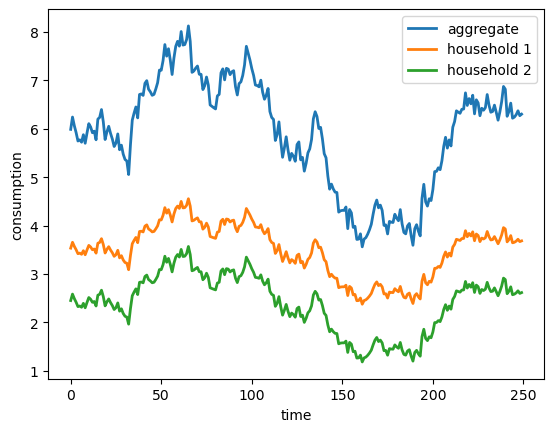
Fig. 23.2 consumption paths#
The next figure plots the limited-markets bond adjustment and confirms that the adjustments sum to approximately zero.
fig, ax = plt.subplots()
ax.plot(paths["k_hat"][0, t0:t0+T_plot], lw=2, label="household 1")
ax.plot(paths["k_hat"][1, t0:t0+T_plot], lw=2, label="household 2")
ax.plot(paths["k_hat"][:, t0:t0+T_plot].sum(axis=0), lw=2, label="sum")
ax.axhline(0.0, color="k", lw=1, alpha=0.5)
ax.set_xlabel("time")
ax.set_ylabel("bond position")
ax.legend()
plt.show()
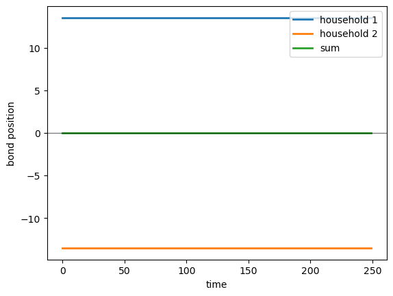
Fig. 23.3 bond position adjustments#
Our final check is to verify that the bond positions sum to zero at all times, confirming that the limited-markets implementation is self-financing
np.max(np.abs(paths["k_hat"].sum(axis=0)))
np.float64(3.552713678800501e-14)
23.6. Example: many-household Gorman economies#
We now extend the two-household example to an economy with many households.
23.6.1. Specification#
The exogenous state vector is
where \(J\) is the number of households and \(J_a\) is the number of “absorbing” households (defined below).
The first three components track a constant and the “ghost” aggregate endowment process. The components \(\{\eta_{j,t}\}_{j=J_a+1}^J\) are idiosyncratic endowment states for the non-absorbing households. The components \(\{\xi_{j,t}\}_{j=1}^J\) are idiosyncratic preference-shock states (often set to zero in experiments).
The aggregate endowment follows an AR(2) process:
where \(w_{1,t+1}\) is the aggregate innovation (the first component of \(w_{t+1}\)) and we can set the \(\rho_j\)’s to capture persistent aggregate fluctuations.
Let \(J_a\) denote the number of “absorbing” households. For households \(j > J_a\), individual endowments are
The first \(J_a\) households absorb the negative of all idiosyncratic endowment shocks to ensure aggregation:
This construction ensures that
Imposing \(\sum_{j=1}^J \phi_j = 1\) gives
To activate the assumptions behind our limited-markets arrangement for implementing an Arrow-Debreu allocation, we silence preference shocks by setting:
where the \(\xi_{j,t}\) processes can be silenced by setting their innovation loadings to zero.
To complete the specification, we let the idiosyncratic states follow AR(1) laws of motion (all innovations are components of the i.i.d. vector \(w_{t+1}\) in \(z_{t+1} = A_{22} z_t + C_2 w_{t+1}\)):
and
Here \(\varepsilon^{d}_{j,t+1}\) and \(\varepsilon^{b}_{j,t+1}\) are mean-zero, unit-variance innovations (components of \(w_{t+1}\)). Setting \(\rho^{d}_j = 0\) (or \(\rho^{b}_j = 0\)) recovers i.i.d. shocks.
def build_gorman_extended(
    n,
    rho1, rho2, sigma_a,
    alphas, phis, sigmas,
    b_bar, gammas,
    rho_idio=0.0,
    rho_pref=0.0,
    n_absorb=None,
):
    """
    Extended version that includes idiosyncratic shocks as state variables,
    allowing the full heterogeneous dynamics to be captured.

    The state vector is:
    z_t = [1, d_{a,t}, d_{a,t-1}, eta_{n_absorb+1,t},
            ..., eta_{n,t}, xi_{1,t}, ..., xi_{n,t}]

    The first n_absorb households absorb the negative sum
    of all idiosyncratic shocks to ensure shocks sum to zero:
    sum_{j=1}^{n_absorb} (-1/n_absorb * sum_{k>n_absorb} eta_k)
    + sum_{k>n_absorb} eta_k = 0

    Each household k > n_absorb has its own idiosyncratic endowment shock
    eta_{k,t} following an AR(1):

        eta_{k,t+1} = rho_idio[k] * eta_{k,t} + sigma_k * w_{k,t+1}

    with rho_idio = 0 recovering i.i.d. shocks (AR(0)).

    Preference shocks xi_{j,t} are included for each household but
    can be set to zero if desired.
    """
    alphas = np.asarray(alphas).reshape(-1)
    phis = np.asarray(phis).reshape(-1)
    sigmas = np.asarray(sigmas).reshape(-1)
    gammas = np.asarray(gammas).reshape(-1)

    assert len(alphas) == len(phis) == len(sigmas) == len(gammas) == n

    # Default: 10% of households absorb shocks (at least 1)
    if n_absorb is None:
        n_absorb = max(1, n // 10)
    n_absorb = int(n_absorb)
    if n_absorb < 1 or n_absorb >= n:
        raise ValueError(
            f"n_absorb must be in [1, n-1], got {n_absorb} with n={n}")

    # Dimensions
    n_idio = n - n_absorb       # eta_{n_absorb+1}, ..., eta_n
    n_pref = n                  # xi_1, ..., xi_n
    nz = 3 + n_idio + n_pref
    nw = 1 + n_idio + n_pref    # aggregate + idio + pref shocks

    # Persistence parameters
    rho_idio = np.asarray(rho_idio, dtype=float)
    if rho_idio.ndim == 0:
        rho_idio = np.full(n_idio, float(rho_idio))
    if rho_idio.shape != (n_idio,):
        raise ValueError(
        f"rho_idio must be scalar or shape ({n_idio},), got {rho_idio.shape}")

    rho_pref = np.asarray(rho_pref, dtype=float)
    if rho_pref.ndim == 0:
        rho_pref = np.full(n_pref, float(rho_pref))
    if rho_pref.shape != (n_pref,):
        raise ValueError(
        f"rho_pref must be scalar or shape ({n_pref},), got {rho_pref.shape}")

    # A22: transition matrix
    A22 = np.zeros((nz, nz))
    A22[0, 0] = 1.0           # constant
    A22[1, 1] = rho1          # d_{a,t} AR(2) first coef
    A22[1, 2] = rho2          # d_{a,t} AR(2) second coef
    A22[2, 1] = 1.0           # lag transition
    for j in range(n_idio):
        A22[3 + j, 3 + j] = rho_idio[j]
    for j in range(n_pref):
        A22[3 + n_idio + j, 3 + n_idio + j] = rho_pref[j]

    # C2: shock loading
    C2 = np.zeros((nz, nw))
    C2[1, 0] = sigma_a
    for j in range(n_idio):
        # Map to households n_absorb+1, ..., n
        C2[3 + j, 1 + j] = sigmas[n_absorb + j]
    for j in range(n_pref):
        C2[3 + n_idio + j, 1 + n_idio + j] = gammas[j]  # gamma_j -> xi_j

    # Ud_per_house: endowment loading
    # First n_absorb households:
    # d_{jt} = alpha_j + phi_j * d_{a,t} - (1/n_ab) * sum_{k>n_ab} eta_{k,t}
    # Remaining households k > n_absorb:
    # d_{kt} = alpha_k + phi_k * d_{a,t} + eta_{k,t}
    Ud_per_house = []
    for j in range(n):
        block = np.zeros((2, nz))
        block[0, 0] = alphas[j]    # constant
        block[0, 1] = phis[j]      # loading on d_{a,t}

        if j < n_absorb:
            for k in range(n_idio):
                block[0, 3 + k] = -1.0 / n_absorb
        else:
            block[0, 3 + (j - n_absorb)] = 1.0

        Ud_per_house.append(block)

    Ud = sum(Ud_per_house)

    # Ub_per_house: bliss loading
    # b_{jt} = b_bars[j] + xi_{j,t}
    # b_bar can be scalar (same for all) or array (household-specific)
    b_bars = np.atleast_1d(b_bar)
    if b_bars.size == 1:
        b_bars = np.full(n, float(b_bars[0]))

    Ub_per_house = []
    for j in range(n):
        row = np.zeros((1, nz))
        row[0, 0] = b_bars[j]         # household-specific bliss
        row[0, 3 + n_idio + j] = 1.0  # loading on xi_j (zeroed if gammas=0)
        Ub_per_house.append(row)

    Ub = sum(Ub_per_house)

    # Initial state
    x0 = np.zeros((nz, 1))
    x0[0, 0] = 1.0  # constant = 1

    return A22, C2, Ub, Ud, Ub_per_house, Ud_per_house, x0
23.6.2. 100-household economy#
We now instantiate a 100-household version of the preceding economy.
We use the same technology and preference parameters.
# Technology and preference parameters
ϕ_1 = 1e-5
γ_1 = 0.1
δ_k = 0.95
β = 1.0 / (γ_1 + δ_k)

θ_k = 1.0
δ_h = 0.0
θ_h = 0.0
Λ = 0.0
Π_h = 1.0

Φ_c = np.array([[1.0], [0.0]])
Φ_g = np.array([[0.0], [1.0]])
Φ_i = np.array([[1.0], [-ϕ_1]])
Γ = np.array([[γ_1], [0.0]])
We set household-specific parameters below and impose \(\sum_j \phi_j = 1\).
rng = np.random.default_rng(42)
N = 100

# Aggregate endowment process parameters
ρ1 = 0.95
ρ2 = 0.0
σ_a = 0.5


# Mean endowments α_j and aggregate exposure φ_j
αs = rng.uniform(3.0, 5.0, N)
φs_raw = rng.uniform(0.5, 1.5, N)
φs = φs_raw / np.sum(φs_raw)  # normalize so Σ φ_j = 1

# Rank households by mean endowment to assign idiosyncratic risk
wealth_rank_proxy = np.argsort(np.argsort(αs))
wealth_pct_proxy = (wealth_rank_proxy + 0.5) / N
poorness = 1.0 - wealth_pct_proxy

# First n_absorb households absorb idiosyncratic shocks
n_absorb = 50

# Poorer households face larger, more persistent idiosyncratic shocks
σ_idio_min, σ_idio_max = 0.2, 5.0
σs = σ_idio_min + (σ_idio_max - σ_idio_min) * (poorness ** 2.0)
ρ_idio_min, ρ_idio_max = 0.0, 0.94
ρ_idio = ρ_idio_min + (ρ_idio_max - ρ_idio_min) * (poorness[n_absorb:] ** 1.0)

# Preference shocks are muted
# Bliss points scale with endowment so high-α households want more consumption
b_bar_base = 5.0
b_bars = b_bar_base * (αs / αs.mean())  # household-specific bliss points
γs_pref = np.zeros(N)
ρ_pref = 0.0

A22, C2, Ub, Ud, Ub_list, Ud_list, x0 = build_gorman_extended(
    n=N,
    rho1=ρ1, rho2=ρ2, sigma_a=σ_a,
    alphas=αs, phis=φs, sigmas=σs,
    b_bar=b_bars, gammas=γs_pref,
    rho_idio=ρ_idio, rho_pref=ρ_pref,
    n_absorb=n_absorb,
)

print(f"sum(φs) = {np.sum(φs):.6f} (should be 1.0)")
sum(φs) = 1.000000 (should be 1.0)
info_ar1 = (A22, C2, Ub, Ud)
pref_ar1 = (np.array([[β]]),
            np.array([[Λ]]),
            np.array([[Π_h]]),
            np.array([[δ_h]]),
            np.array([[θ_h]]))
tech_ar1 = (Φ_c, Φ_g, Φ_i, Γ,
            np.array([[δ_k]]),
            np.array([[θ_k]]))

paths, econ = solve_model(info_ar1, tech_ar1, pref_ar1,
                    Ub_list, Ud_list, γ_1, Λ, z0=x0)
print(f"State dimension: {A22.shape[0]}, shock dimension: {C2.shape[1]}")
print(f"Aggregate: ρ_1={ρ1:.3f}, ρ_2={ρ2:.3f}, σ_a={σ_a:.2f}")
print(f"Endowments: α in [{np.min(αs):.2f}, {np.max(αs):.2f}]")
State dimension: 153, shock dimension: 151
Aggregate: ρ_1=0.950, ρ_2=0.000, σ_a=0.50
Endowments: α in [3.01, 4.95]
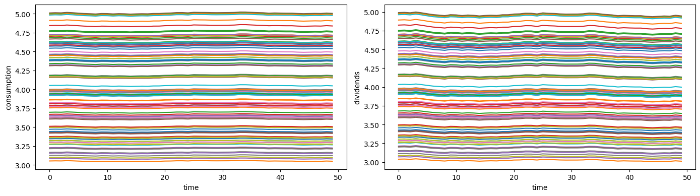
The next plots show household consumption and dividend paths after discarding the initial burn-in period.
T_plot = 50

fig, axes = plt.subplots(1, 2, figsize=(14, 4))

axes[0].plot(paths["c_j"][:, t0:t0+T_plot].T)
axes[0].set_xlabel("time")
axes[0].set_ylabel("consumption")

axes[1].plot(paths["d_share"][:, t0:t0+T_plot].T)
axes[1].set_xlabel("time")
axes[1].set_ylabel("dividends")

plt.tight_layout()
plt.show()
23.7. State-space representation#
23.7.1. Closed-loop state-space system#
We can use our DLE tools first to solve the representative-household social planning problem and represent equilibrium quantities as a linear closed-loop state-space system that takes the usual Chapter 5 Hansen and Sargent [2013] form
where the aggregate state vector is
with \(h_{t-1}\) the aggregate household service stock, \(k_{t-1}\) the aggregate capital stock, and \(z_t\) the exogenous state (constant, aggregate endowment states, and idiosyncratic shock states).
Any equilibrium quantity is a linear function of the state.
The quantecon.DLE module provides selection matrices \(S_\bullet\) such that:
We can stack these to form a measurement matrix:
A0 = econ.A0
C = econ.C

G = np.vstack([
    econ.Sc,
    econ.Sg,
    econ.Si,
    econ.Sh,
    econ.Sk,
    econ.Sd,
    econ.Sb,
    econ.Ss,
])

# Extract dimensions for proper slicing
n_h = np.atleast_2d(econ.thetah).shape[0]
n_k = np.atleast_2d(econ.thetak).shape[0]
n_endo = n_h + n_k  # endogenous state dimension
With the state-space representation, we can compute impulse responses to show how shocks propagate.
To trace the impulse response to shock \(j\), we set shock_idx=j which selects column \(j\) of the loading matrix \(C\).
This creates an initial state \(x_0 = C e_j \sigma\) where \(e_j\) is the \(j\)-th standard basis vector and \(\sigma\) is the shock size.
We then iterate forward with \(x_{t+1} = A_0 x_t\) and compute observables via \(y_t = G x_t\).
def compute_irf(A0, C, G, shock_idx, T=50, shock_size=1.0):
    """Compute impulse response to shock shock_idx with given shock size."""
    n_x = A0.shape[0]
    n_w = C.shape[1]

    x_path = np.zeros((n_x, T))
    y_path = np.zeros((G.shape[0], T))

    w0 = np.zeros(n_w)
    w0[shock_idx] = shock_size
    x_path[:, 0] = C @ w0
    y_path[:, 0] = G @ x_path[:, 0]

    for t in range(1, T):
        x_path[:, t] = A0 @ x_path[:, t-1]
        y_path[:, t] = G @ x_path[:, t]

    return x_path, y_path

n_h = np.atleast_2d(econ.thetah).shape[0]
n_k = np.atleast_2d(econ.thetak).shape[0]

idx_da = n_h + n_k + 1
T_irf = 50
shock_size = 1.0
irf_x, irf_y = compute_irf(A0, C, G, shock_idx=0, T=T_irf, shock_size=shock_size)
idx_k = 4  # index of capital in stacked observable vector G @ x


da_irf = irf_x[idx_da, :]

fig, axes = plt.subplots(1, 2, figsize=(14, 4))


axes[0].plot(irf_y[idx_k, :], lw=2)
axes[0].set_xlabel('time')
axes[0].set_ylabel('capital')

axes[1].plot(da_irf, lw=2)
axes[1].set_xlabel('time')
axes[1].set_ylabel(r'$d_{a,t}$')


plt.tight_layout()
plt.show()
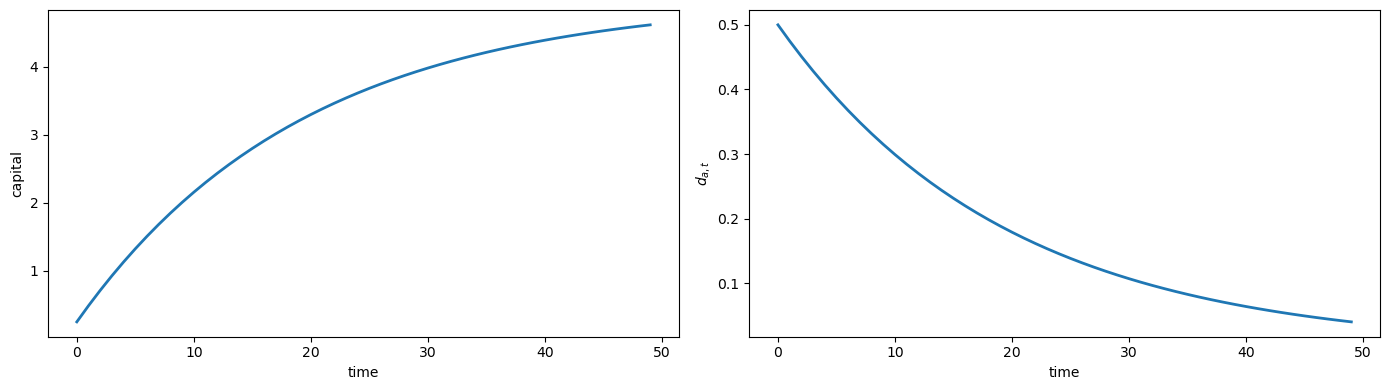
The aggregate endowment shock \(d_{a,t}\) follows an AR(1) process with \(\rho_1 = 0.95\), so after the initial impact it decays monotonically toward zero as \(0.95^t\).
By contrast, capital is an endogenous stock that accumulates when the planner smooths consumption.
The positive endowment shock increases resources temporarily, but Hall-style preferences imply the planner saves part of the windfall rather than consuming it immediately.
This causes capital to rise as \(d_{a,t}\) falls – this is permanent income logic at work.
Next, we examine whether the household consumption and endowment paths generated by the simulation obey the Gorman sharing rule
c_j_t0 = paths["c_j"][..., t0:]
d_j_t0 = paths["d_share"][..., t0:]

c_panel = np.asarray(c_j_t0 - c_j_t0.mean(axis=0))  # (N, T - t0)
d_panel = np.asarray(d_j_t0 - d_j_t0.mean(axis=0))  # (N, T - t0)
assert c_panel.shape == d_panel.shape

# Plot aggregate endowment and individual household endowments
d_agg = paths["d"][0, t0:]
d_households = d_j_t0

T_plot = min(500, d_agg.shape[0])
time_idx = np.arange(T_plot)
n_to_plot = 1


fig, axes = plt.subplots(2, 1, figsize=(14, 8))

# Top panel: Aggregate endowment
axes[0].plot(time_idx, d_agg[:T_plot], linewidth=2.5, color='C0',
        label='Aggregate endowment $d_t$')
axes[0].set_title('Aggregate Endowment')
axes[0].set_ylabel('endowment')
axes[0].legend()

# Also plot the mean across households
d_mean = d_households[:, :T_plot].mean(axis=0)
axes[1].plot(time_idx, d_mean, linewidth=2.5, color='black', linestyle='--',
            label=f'Mean across {d_households.shape[0]} households', alpha=0.8)

axes[1].set_title(f'Average of Individual Household Endowments')
axes[1].set_xlabel('time (after burn-in)')
axes[1].set_ylabel('endowment')
axes[1].legend(loc='upper right', ncol=2)

plt.tight_layout()
plt.show()
Indeed, the average of individual household endowments tracks the aggregate endowment process, confirming that the construction of the idiosyncratic shocks and absorbing households works as intended.
23.8. Redistributing by adjusting Pareto weights#
This section analyzes Pareto-efficient tax-and-transfer schemes by starting with competitive equilibrium allocations and using a specific set of nonnegative Pareto weights that sum to one.
Note
There are various tax-and-transfer schemes that would deliver such efficient redistributions, but in terms of what interests us in this example, they are all equivalent.
23.8.1. Redistribution via Pareto weights#
The sharing rule (23.11) can be written as \(c_{jt} - \chi_{jt} = \mu_j (c_t - \chi_t)\), where \(\mu_j\) is household \(j\)’s Pareto weight.
Define the Pareto weight \(\lambda_j := \mu_j\), with \(\sum_{j=1}^J \lambda_j = 1\).
Consider redistributing consumption by choosing new weights \(\{\lambda_j^*\}\) satisfying \(\lambda_j^* \geq 0\) and \(\sum_j \lambda_j^* = 1\).
The new allocation \(c_{jt} - \chi_{jt} = \lambda_j^* (c_t - \chi_t)\) preserves aggregate dynamics \((c_t, k_t)\) while reallocating consumption across households.
Let \(R := \delta_k + \gamma_1\).
For a given Pareto-weight vector \(\omega\), household \(j\)’s assets are \(a_{j,t} := \omega_j k_t + \hat{k}_{j,t}\) and income is
We want to compare pre- and post-redistribution consumption and income.
Let \(\mu := \{\mu_j\}_{j=1}^J\) denote the original competitive equilibrium Pareto weights, and let \(\lambda^* := \{\lambda_j^*\}_{j=1}^J\) denote the redistributed weights.
We write \(y^{pre}_{j,t} = y_{j,t}(\mu)\) and \(y^{post}_{j,t} = y_{j,t}(\lambda^*)\), then compare consumption to income using percentile plots.
To implement a redistribution from \(\mu\) to \(\lambda^*\), we construct new Pareto weights \(\{\lambda_j^*\}_{j=1}^J\) that:
Lower the weights for low-\(j\) types (wealthier households in our ordering)
Increase the weights for high-\(j\) types (less wealthy households)
Leave middle-\(j\) types relatively unaffected
Preserve the constraint \(\sum_{j=1}^J \lambda_j^* = 1\)
We choose to implement these steps by using a smooth transformation.
Let \(\{\lambda_j\}_{j=1}^J\) denote the original competitive equilibrium Pareto weights (sorted in descending order). Define the redistribution function:
where:
\(j \in \{1, \ldots, J\}\) is the household index
\(\alpha > 0\) controls the overall magnitude of redistribution
\(\beta\) controls the progressivity (higher \(\beta\) concentrates redistribution more strongly in the tails)
Post-redistribution Pareto weights are:
where \(\bar{\lambda} = J^{-1}\) is the equal-weight benchmark.
To ensure that our weights sum to unity, we normalize:
def create_redistributed_weights(λ_orig, α=0.5, β=2.0):
    """Create more egalitarian Pareto weights via smooth redistribution."""
    λ_orig = np.asarray(λ_orig, dtype=float)
    J = len(λ_orig)
    if J == 0:
        raise ValueError("λ_orig must be non-empty")
    if J == 1:
        return np.array([1.0])
    λ_bar = 1.0 / J
    j_indices = np.arange(J)
    f_j = j_indices / (J - 1)
    dist_from_median = np.abs(f_j - 0.5) / 0.5
    τ_j = np.clip(α * (dist_from_median ** β), 0.0, 1.0)
    λ_tilde = λ_orig + τ_j * (λ_bar - λ_orig)
    λ_star = λ_tilde / λ_tilde.sum()
    return λ_star
Let’s plot the effect of redistribution on the Pareto weights in our 100-household economy
μ_values = paths["μ"]
idx_sorted = np.argsort(-μ_values)
λ_orig_sorted = μ_values[idx_sorted]

red_α = 0.8
red_β = 0.0

λ_star_sorted = create_redistributed_weights(λ_orig_sorted, α=red_α, β=red_β)

# Map redistributed weights back to the original household ordering
λ_star = np.empty_like(μ_values, dtype=float)
λ_star[idx_sorted] = λ_star_sorted

fig, axes = plt.subplots(1, 2, figsize=(14, 5))

n_plot = len(λ_orig_sorted)
axes[0].plot(λ_orig_sorted[:n_plot], 'o-',
            label=r'original $\lambda_j$', alpha=0.7, lw=2)
axes[0].plot(λ_star_sorted[:n_plot], 's-',
            label=r'redistributed $\lambda_j^*$', alpha=0.7, lw=2)
axes[0].axhline(1.0 / len(λ_orig_sorted), color='k', linestyle='--',
            label=f'equal weight (1/{len(λ_orig_sorted)})', alpha=0.5, lw=2)
axes[0].set_xlabel(r'household index $j$ (sorted by $\lambda$)')
axes[0].set_ylabel('Pareto weight')
axes[0].legend()

Δλ_sorted = λ_star_sorted - λ_orig_sorted
axes[1].bar(range(n_plot), Δλ_sorted[:n_plot], alpha=0.7,
            color=['g' if x > 0 else 'r' for x in Δλ_sorted[:n_plot]])
axes[1].axhline(0, color='k', linestyle='-', lw=2)
axes[1].set_xlabel(r'household index $j$ (sorted by $\lambda$)')
axes[1].set_ylabel(r'$\lambda_j^* - \lambda_j$')

plt.tight_layout()
plt.show()
Once we have the redistributed Pareto weights, we can compute the new household consumption and income paths.
The function below computes household consumption and income under given Pareto weights
def allocation_from_weights(paths, econ,
                            U_b_list, weights, γ_1, Λ, h0i=None,
                            original_weights=None):
    """
    Compute household consumption and income under given Pareto weights.
    """

    weights = np.asarray(weights).reshape(-1)
    N = len(weights)

    # For χ computation, use original weights if provided
    if original_weights is None:
        weights_for_chi = weights
    else:
        weights_for_chi = np.asarray(original_weights).reshape(-1)

    # Extract aggregate paths
    x_path = paths["x_path"]
    c_agg = paths["c"]
    d_agg = paths["d"]
    k_agg = paths["k"]
    z_path = paths["z_path"]

    _, T = c_agg.shape

    # Get parameters
    Θ_h = np.atleast_2d(econ.thetah)
    Δ_h = np.atleast_2d(econ.deltah)
    Π_h = np.atleast_2d(econ.pih)
    Λ = np.atleast_2d(Λ)
    n_h = Θ_h.shape[0]

    δ_k = float(np.asarray(econ.deltak).squeeze())
    R = δ_k + float(γ_1)

    Π_inv = np.linalg.inv(Π_h)
    A_h = Δ_h - Θ_h @ Π_inv @ Λ
    B_h = Θ_h @ Π_inv

    if h0i is None:
        h0i = np.zeros((n_h, 1))

    # Compute household allocations
    c_j = np.zeros((N, T))
    χ_tilde = np.zeros((N, T))
    k_hat = np.zeros((N, T))

    for j in range(N):
        U_bj = np.asarray(U_b_list[j], dtype=float)
        b_agg = econ.Sb @ x_path
        # Use weights_for_chi for b_tilde: keeps χ fixed during redistribution
        b_tilde = U_bj @ z_path - weights_for_chi[j] * b_agg

        η = np.zeros((n_h, T + 1))
        η[:, 0] = np.asarray(h0i).reshape(-1)
        # At t=0, assume η_{-1} = 0
        χ_tilde[j, 0] = (Π_inv @ b_tilde[:, 0]).squeeze()
        for t in range(1, T):
            χ_tilde[j, t] = (
                -Π_inv @ Λ @ η[:, t - 1] + Π_inv @ b_tilde[:, t]).squeeze()
            η[:, t] = (A_h @ η[:, t - 1] + B_h @ b_tilde[:, t]).squeeze()

        c_j[j] = (weights[j] * c_agg[0] + χ_tilde[j]).squeeze()

        # Solve for bond path by backward iteration from terminal condition.
        if abs(R - 1.0) >= 1e-14:
            k_hat[j, -1] = χ_tilde[j, -1] / (R - 1.0)
            for t in range(T - 1, 0, -1):
                k_hat[j, t - 1] = (k_hat[j, t] + χ_tilde[j, t]) / R

    # Compute income
    k_share = weights[:, None] * k_agg[0, :]
    a_total = k_share + k_hat

    # Lagged assets
    a_lag = np.concatenate([a_total[:, [0]], a_total[:, :-1]], axis=1)

    # Net income: dividend share + asset return
    y_net = weights[:, None] * d_agg[0, :] + (R - 1) * a_lag

    return {"c": c_j, "y_net": y_net,
            "χ_tilde": χ_tilde, "k_hat": k_hat,
            "a_total": a_total}
μ_values = np.asarray(paths["μ"]).reshape(-1)

R = float(δ_k + γ_1)

# Redistribution parameters (same as visualization above)
red_α = 0.8
red_β = 0.0

idx_sorted = np.argsort(-μ_values)
λ_orig_sorted = μ_values[idx_sorted]

λ_star_sorted = create_redistributed_weights(λ_orig_sorted, α=red_α, β=red_β)
λ_star = np.empty_like(μ_values, dtype=float)
λ_star[idx_sorted] = λ_star_sorted

h0i_alloc = np.array([[0.0]])

pre = allocation_from_weights(paths, econ,
                Ub_list, μ_values, γ_1, Λ, h0i_alloc)

# For post-redistribution: use λ_star for proportional share, but keep χ fixed
# that is to say preferences don't change with taxes
post = allocation_from_weights(paths, econ,
                Ub_list, λ_star, γ_1, Λ, h0i_alloc,
                original_weights=μ_values)

c_pre = pre["c"][:, t0:]
y_pre = pre["y_net"][:, t0:]
c_post = post["c"][:, t0:]
y_post = post["y_net"][:, t0:]

def _pct(panel, ps=(90, 50, 10)):
    return np.percentile(panel, ps, axis=0)

T_ts = min(500, c_pre.shape[1] - 50)
t = t0 + np.arange(T_ts)

y_pre_pct = _pct(y_pre[:, :T_ts])
y_post_pct = _pct(y_post[:, :T_ts])
c_pre_pct = _pct(c_pre[:, :T_ts])
c_post_pct = _pct(c_post[:, :T_ts])

fig, ax = plt.subplots(1, 3, figsize=(14,  6), sharey=True)

ax[0].plot(t, y_pre_pct[0], label="p90", lw=2)
ax[0].plot(t, y_pre_pct[1], label="p50", lw=2)
ax[0].plot(t, y_pre_pct[2], label="p10", lw=2)
ax[0].set_xlabel("$t$", fontsize=20)
ax[0].set_ylabel(r"$y^{pre}$", fontsize=20)

ax[1].plot(t, y_post_pct[0], label="p90", lw=2)
ax[1].plot(t, y_post_pct[1], label="p50", lw=2)
ax[1].plot(t, y_post_pct[2], label="p10", lw=2)
ax[1].set_xlabel("$t$")
ax[1].set_ylabel(r"$y^{post}$", fontsize=20)

ax[2].plot(t, c_post_pct[0], label="p90", lw=2)
ax[2].plot(t, c_post_pct[1], label="p50", lw=2)
ax[2].plot(t, c_post_pct[2], label="p10", lw=2)
ax[2].set_xlabel("$t$")
ax[2].set_ylabel(r"$c^{post}$", fontsize=20)

handles, labels = ax[0].get_legend_handles_labels()

fig.legend(
    handles,
    labels,
    loc="upper center",
    ncol=3,
    frameon=False,
    bbox_to_anchor=(0.5, 1.1),
)

plt.tight_layout()
plt.show()
The figures reveal a striking reduction in income and consumption inequality after redistribution.
Also, notice how insurance smooths consumption relative to income, especially for lower-percentile households.
The post-tax-and-transfer income path exhibits less volatility for the lower percentiles compared to the pre-tax-and-transfer income.