
27. Dynamic Supply and Demand Curves#
27.1. Overview#
This lecture constructs dynamic supply and demand curves for a market for a single good.
In this lecture, we shall
set up a market in which a representative supplier and a representative demander each solve a linear-quadratic dynamic optimization problem,
derive dynamic supply and demand curves by factoring each agent’s Euler equation into stable and unstable roots, then solving stable roots backwards and unstable roots forwards,
recast the optimization problem faced by each side of the market within a rational expectations equilibrium as an optimal linear regulator, using an instance of the “Big \(X\), little \(x\)” device used throughout modern macroeconomics, and
explain why a vector autoregression fit to a history of equilibrium prices and quantities can give a distorted picture of the shocks that drive suppliers’ and demanders’ information sets — a difficulty that afflicts Christopher Sims’s [Sims, 1980] innovation accounting more generally.
Along the way we obtain representations of dynamic supply and demand curves both outside and inside a rational expectations equilibrium.
This lecture also revisits an issue discussed in Shock Non Invertibility, which described a shock-invertibility problem inside a permanent income model.
This lecture studies the same problem in the context of a model of a single competitive market for a good whose price and quantity are both observed.
The model is a version of a discrete-time example in Lars Peter Hansen and Thomas J. Sargent’s “Two difficulties in interpreting vector autoregressions” [Hansen and Sargent, 1991].
In addition to what’s in Anaconda, this lecture uses the quantecon library.
!pip install --upgrade quantecon
We’ll make these imports:
import numpy as np
import quantecon as qe
import matplotlib.pyplot as plt
from quantecon import LQ
27.2. The setting#
There is a competitive market for a single good produced in quantity \(q_t\) and sold at price \(p_t\).
A representative supplier and a representative demander each solve a linear-quadratic dynamic problem, taking the market price \(\{p_t\}\) as an exogenous stochastic process.
The supplier chooses \(\{q_t\}\) to maximize
It earns revenue \(p_t q_t\), pays a quadratic cost of adjusting output through the term \(\tfrac{g_s}{2}(q_t - q_{t-1})^2\), and is buffeted by a serially correlated cost shock \(s_t\).
The demander chooses \(\{q_t\}\) to maximize
It pays \(p_t q_t\) for the good, values a service flow \(a(L)q_t\) generated by current and past purchases through a durable-services technology \(a(L) = a_0 + a_1 L + a_2 L^2 + a_3 L^3 + a_4 L^4\), and is shifted by a demand shock \(d_t\).
Here \(\beta\) is a discount factor and \(L\) is the lag operator, \(L q_t = q_{t-1}\).
Differentiating (27.1) and (27.2) with respect to \(q_t\) gives the supplier’s and demander’s Euler equations
where \(L^{-1}\) is the forward operator, \(L^{-1} q_t = q_{t+1}\).
The supply and demand shocks are serially correlated,
with \(B_s(z), B_d(z)\) having zeros outside the unit circle and \(w_{st}, w_{dt}\) mutually uncorrelated white noises that the agents observe.
The white noise fundamental for the agents is \(\epsilon_t = (w_{st}, w_{dt})\).
We study the market at the parameters
Notice that the supplier’s adjustment cost \(g_s = 10\) is a hundred times the demander’s \(g_d = 0.1\).
Quantity will therefore adjust sluggishly — a feature that turns out to be the source of the difficulty in interpreting a vector autoregression fit to \((q_t, p_t)\).
h_s = h_d = 1.0
g_s, g_d = 10.0, 0.1
β = 1 / 1.05
a = np.array([1, .8, .6, .4, .2])       # a(L): coefficients a0..a4

# MA polynomials for the shocks (coefficients on L^0..L^3)
B_d = np.convolve(np.convolve([1, .6], [1, .4]), [1, .2])
B_s = np.convolve(np.convolve([1, -.8], [1, .4]), [1, .2])

σ_s2, σ_d2 = 0.5, 4.0                   # shock variances
27.3. Dynamic supply and demand curves#
Before imposing market clearing it is illuminating to solve each agent’s Euler equation separately.
Each is an expectational difference equation in \(q_t\), and each is solved by the standard device of Classical Control with Linear Algebra:
factor the characteristic operator into a stable root and an unstable root, solve the stable root backwards into a feedback on lagged quantities, and solve the unstable root forwards into a geometric sum of expected future variables.
The two solutions are dynamic supply and demand curves.
27.3.1. The dynamic supply curve#
Write the supplier’s Euler equation (27.3) as \(E_t\,\phi_s(L)\,q_t = p_t - s_t\), with characteristic operator
Because \(\phi_s\) is symmetric under \(L \mapsto \beta L^{-1}\), the roots of its symbol come in a reciprocal pair \((\delta_s,\ \beta/\delta_s)\), the two solutions of the supplier’s characteristic equation
Let \(\delta_s\) be the smaller root, \(|\delta_s| < \sqrt{\beta} < 1\).
# supplier's characteristic equation: z^2 - [(1+β) + h_s/g_s] z + β = 0
supply_roots = np.roots([1, -((1 + β) + h_s / g_s), β])
δ_s = min(supply_roots, key=abs)

print(f"supply roots         : {np.sort(supply_roots)}")
print(f"δ_s                  : {δ_s:.4f}   (sqrt(β) = {np.sqrt(β):.4f})")
print(f"δ_s / β              : {δ_s / β:.4f}")
supply roots         : [0.70888    1.34350096]
δ_s                  : 0.7089   (sqrt(β) = 0.9759)
δ_s / β              : 0.7443
The operator factors as
an unstable forward factor \((1-\delta_s L^{-1})\) and a stable backward factor \((1-\tfrac{\delta_s}{\beta}L)\).
Solving the forward root forward — a geometric sum of expected future variables, exactly as in Classical Control with Linear Algebra — and reading the backward root as a feedback on the lag of \(q\), the supplier’s Euler equation becomes the dynamic supply curve
Current quantity supplied is a geometrically declining feedback on its own lag \(q_{t-1}\) plus the conditional expectation of a discounted geometric sum of future prices \(p_{t+j}\) and future supply shocks \(s_{t+j}\).
Higher expected future prices raise current supply; a higher expected cost shock lowers it.
Only the single lag \(q_{t-1}\) appears, because the supplier’s adjustment cost penalizes \((1-L)q_t\) one period at a time.
27.3.2. The dynamic demand curve#
The demander’s Euler equation (27.4) is \(E_t\,\phi_d(L)\,q_t = -(p_t + d_t)\), with characteristic operator
Since \(a(L)\) has degree four, \(\phi_d\) is again symmetric under \(L \mapsto \beta L^{-1}\), but now its symbol has eight roots in four reciprocal pairs \((\delta_{d,i},\ \beta/\delta_{d,i})\), \(i = 1,\dots,4\).
Collecting the four stable roots \(|\delta_{d,i}| < \sqrt{\beta}\), the factorization is
with \(\nu_d > 0\) a normalizing constant.
We find the eight roots numerically.
The symbol \(\phi_d(z) = h_d + g_d\, a(z)\, a(\beta/z)\) is a Laurent polynomial; multiplying by \(z^4\) turns it into an ordinary degree-8 polynomial whose roots we can read off.
# a(z) as an ordinary polynomial (highest power first)
a_z = np.poly1d(a[::-1])
# z^4 * a(β/z): coefficients of z^4 .. z^0 are a0, a1 β, ..., a4 β^4
a_βz = np.poly1d([a[k] * β**k for k in range(5)])

# z^4 * φ_d(z) = h_d z^4 + g_d * a(z) * (z^4 a(β/z))
poly = (g_d * a_z * a_βz).c
poly[4] += h_d
demand_roots = np.roots(poly)

moduli = np.abs(demand_roots)
δ_d = demand_roots[moduli < np.sqrt(β)]                # the four stable roots

print("moduli of the eight roots :", np.round(np.sort(moduli), 4))
print("stable δ_d,i moduli       :", np.round(np.sort(np.abs(δ_d)), 4))
moduli of the eight roots : [0.3026 0.3026 0.3892 0.3892 2.447  2.447  3.1471 3.1471]
stable δ_d,i moduli       : [0.3026 0.3026 0.3892 0.3892]
The four stable roots are two complex-conjugate pairs, of modulus roughly \(0.30\) and \(0.39\).
Reading the backward factor \(c_d(L)\) as a feedback on lags gives the dynamic demand curve
where the \(A_{d,i}\) are the partial-fraction weights of the inverse forward factor.
Now current quantity demanded depends on four lags \(q_{t-1},\dots,q_{t-4}\) — the durable-services technology \(a(L)\) spreads adjustment over four periods — and on a sum of geometric feed-forward terms, one per stable root.
The price terms enter with a negative sign: higher expected future prices lower current demand.
We recover the feedback coefficients \(\gamma_{d,k}\) from the stable roots.
# c_d(L) = prod_i (1 - (δ_d,i / β) L) = 1 - Σ γ_d,k L^k
c_d = np.array([1.0])
for r in δ_d / β:
    c_d = np.convolve(c_d, [1, -r])
c_d = c_d.real

γ_d = -c_d[1:]
print("γ_d,k =", np.round(γ_d, 4))
γ_d,k = [-0.1174 -0.0792 -0.0447 -0.0169]
The feedback weights \((\gamma_{d,1},\dots,\gamma_{d,4}) \approx (-0.117,\,-0.079,\,-0.045,\,-0.017)\) decline smoothly with the lag.
27.3.3. Both shocks shift both curves#
Taken at face value, the dynamic supply curve (27.8) seems to involve only supply shocks and the dynamic demand curve (27.10) only demand shocks.
But each curve also contains the conditional expectations \(E_t\,p_{t+j}\) of future prices, and in equilibrium the price process is driven by both shocks.
A demand surprise that moves expected future prices therefore shifts the dynamic supply curve, and a supply surprise that moves expected future prices shifts the dynamic demand curve.
It is exactly this dependence on forecasts of future prices — absent from static supply and demand curves — that couples the two sides of the market and makes the equilibrium dynamics richer than a sequence of momentary intersections.
27.4. The equilibrium via a market Euler equation#
The two dynamic curves describe supply and demand for an arbitrary price process.
A rational expectations equilibrium adds two requirements: quantity demanded equals quantity supplied every period, and the price forecasts \(E_t\,p_{t+j}\) that appear in both curves are the ones generated by the equilibrium price process itself.
We impose these requirements directly on the two Euler equations (27.3) and (27.4), combining them into a single market Euler equation for quantities and solving it by the same factorization we used for the individual curves.
Step 1 — drop the conditional expectations and solve each Euler equation for \(p_t\).
Temporarily erase the operator \(E_t\) from the left side of each Euler equation, and solve each for the price:
Step 2 — equate the two prices to get a single market Euler equation in \(q_t\) alone.
Setting (27.11) equal to (27.12) eliminates \(p_t\) and leaves
a two-sided difference equation that involves past, present, and future \(q\)’s together with the two shocks.
Like \(\phi_s\) and \(\phi_d\) separately, the market operator \(\psi\) is symmetric under \(L \mapsto \beta L^{-1}\), so the symbol \(z^4\psi(z)\) is a degree-eight polynomial whose eight roots come in four reciprocal pairs \((\lambda_i,\ \beta/\lambda_i)\).
Step 3 — factor, solve stable roots backwards and unstable roots forwards.
Collecting the four stable roots \(|\lambda_i| < \sqrt{\beta}\) gives the factorization
with \(\nu > 0\) a normalizing constant, \(c(L)\) the stable backward factor, and \(c(\beta L^{-1})\) the forward factor.
Dividing (27.13) by \(\nu \, c(\beta L^{-1})\) solves the unstable roots forwards.
Step 4 — reinstate \(E_t\) in front of the continuation shocks.
The forward operator acts on future values of the exogenous shocks, so we now put \(E_t\) back in front of them, giving the equilibrium law of motion for quantities
where the \(A_i\) are the partial-fraction weights of \(\big[c(\beta L^{-1})\big]^{-1} = \sum_i A_i/(1-\lambda_i L^{-1})\).
The conditional expectations are evaluated with the Hansen–Sargent prediction formula: for a shock \(x_t = B(L)\,w_t\) driven by white noise \(w_t\),
Notice that (27.15) has exactly the shape of the individual dynamic supply and demand curves — a backward-looking feedback on lagged quantities plus geometric feed-forward sums — but now with the combined operator \(\psi\) and the combined forcing \(-(s_t + d_t)\).
The coefficients \(\gamma_k\) are the equilibrium feedback of current quantity on its own four lags.
We build \(\psi\), factor it, and read them off.
# the market operator ψ(z) = φ_s(z) + φ_d(z), times z^4 (a degree-8 polynomial)
a_z = np.poly1d(a[::-1])                             # a(z)
a_βz = np.poly1d([a[k] * β**k for k in range(5)])    # z^4 * a(β/z)
ψ = (g_d * a_z * a_βz).c.copy()          # g_d * a(βL^-1)a(L), highest-first

# add val * z^k to ψ (a degree-8 coefficient vector, highest power first)
def add_power(coef, k, val):
    coef[8 - k] += val

add_power(ψ, 4, h_s + h_d)               # h_s + h_d
add_power(ψ, 4, g_s * (1 + β))           # the g_s(1-βL^-1)(1-L) part:
add_power(ψ, 5, -g_s)                    #   g_s[(1+β) - L - β L^-1]
add_power(ψ, 3, -g_s * β)

roots = np.roots(ψ)
λ = roots[np.abs(roots) < np.sqrt(β)]    # the four stable roots
assert len(λ) == 4

# backward factor c(L) = Π (1 - (λ_i/β) L) = 1 - Σ γ_k L^k
c_mkt = np.array([1.0])
for r in λ / β:
    c_mkt = np.convolve(c_mkt, [1, -r])
γ_mkt = -c_mkt[1:].real

print("market backward-factor feedback γ_k :", np.round(γ_mkt, 4))
market backward-factor feedback γ_k : [ 0.607 -0.0087 -0.0042 -0.0012]
The four stable roots deliver a fourth-order feedback of current quantity on its own past.
Now we complete the forward part and construct the equilibrium responses.
We form the normalizing constant \(\nu\) and the partial-fraction weights \(A_i\), evaluate the feed-forward sums with (27.16), and simulate the moving-average response of \(q_t\) implied by (27.15).
The price then follows from the supply relation (27.11), restoring \(E_t\): \(p_t = s_t + h_s q_t + g_s[(1+\beta)q_t - q_{t-1} - \beta E_t q_{t+1}]\).
Along an impulse response there are no further shocks, so \(E_t q_{t+1} = q_{t+1}\).
ν = (ψ[0] / np.prod(-λ / β)).real        # normalizing constant

# partial-fraction weights
A_pf = np.array([1 / np.prod([1 - λ[k] / λ[i] for k in range(4) if k != i])
                 for i in range(4)])

def hs_predict(B, λ):
    "E_t Σ_j λ^j x_(t+j) = (L B(L) - λ B(λ)) / (L - λ) applied to w_t."
    B = np.asarray(B, dtype=complex)
    # numerator L B(L) - λ B(λ), lowest power first
    num = np.concatenate(([-λ * np.polyval(B[::-1], λ)], B))
    quo, _ = np.polydiv(num[::-1], [1, -λ])   # exact division by (L - λ)
    return quo[::-1].real

def forcing(B):
    "MA coefficients of the feed-forward term -(1/ν) Σ_i A_i (H-S) on w."
    M = sum(A_pf[i] * hs_predict(B, λ[i]) for i in range(4))
    return (-M / ν).real

M_s, M_d = forcing(B_s), forcing(B_d)

def q_response(M, T=27):
    "Response of q to a unit shock, from q_t = Σ γ_k q_(t-k) + M(L) w."
    q = np.zeros(T)
    for t in range(T):
        q[t] = sum(γ_mkt[k - 1] * q[t - k]
                   for k in range(1, 5) if t - k >= 0)
        if t < len(M):
            q[t] += M[t]
    return q

def p_response(q, s_path, T=25):
    "Price from the supply relation; E_t q_(t+1) = q_(t+1) on an IRF path."
    p = np.zeros(T)
    for t in range(T):
        q_lag = q[t - 1] if t else 0.0
        p[t] = (s_path[t] + h_s * q[t]
                + g_s * ((1 + β) * q[t] - q_lag - β * q[t + 1]))
    return p

scale = np.diag([np.sqrt(σ_s2), np.sqrt(σ_d2)])   # shock std devs

q_s, q_d = q_response(M_s), q_response(M_d)
irf_mkt = np.zeros((25, 2, 2))
s_path = np.concatenate([B_s, np.zeros(25)])
irf_mkt[:, 0, 0], irf_mkt[:, 1, 0] = q_s[:25], p_response(q_s, s_path)
irf_mkt[:, 0, 1], irf_mkt[:, 1, 1] = q_d[:25], p_response(q_d, np.zeros(25))
irf_mkt *= scale.diagonal()      # scale each shock by its std dev
We plot the equilibrium responses of quantity and price to the two structural shocks.
fig, axes = plt.subplots(1, 2, figsize=(12, 4))
for col, name in enumerate(["supply shock $w_{st}$", "demand shock $w_{dt}$"]):
    axes[col].plot(irf_mkt[:, 0, col], label="quantity $q_t$")
    axes[col].plot(irf_mkt[:, 1, col], label="price $p_t$")
    axes[col].axhline(0, color="k", lw=0.5)
    axes[col].set_title(f"response to {name}")
    axes[col].set_xlabel("periods")
    axes[col].legend()
plt.tight_layout()
plt.show()
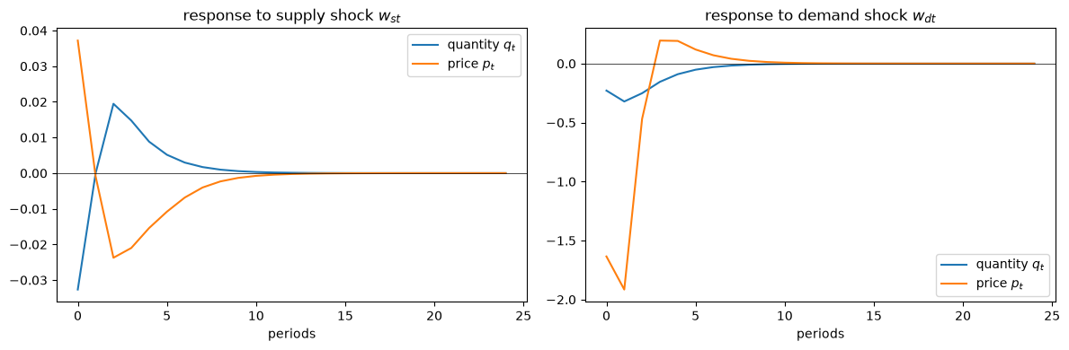
A demand surprise moves the price sharply on impact with only a small quantity response, because the large adjustment cost \(g_s\) prevents the supplier from expanding output quickly.
A supply surprise sends quantity and price off in opposite directions.
In both cases quantity moves slowly — the hallmark of the sluggish adjustment that \(g_s = 10\) builds in.
27.5. The equilibrium from an optimal linear regulator#
We now compute the same equilibrium a second way, as an optimal linear regulator.
This construction also delivers the state-space representation \(X_{t+1} = A_F X_t + C\,w_{t+1}\), \(z_t = G_z X_t\) that we reuse later — for the price-taking regulators and for the Kalman-filter analysis of vector autoregressions.
Because the market objectives are quadratic and the shocks enter linearly, the competitive equilibrium coincides with the allocation chosen by a fictitious planner who maximizes the sum of the two objectives.
The revenue terms \(p_t q_t\) cancel when quantity supplied equals quantity demanded, so the planner maximizes
The equilibrium price is then the common marginal valuation; reading it off the supplier’s Euler equation (27.3),
We solve the planner’s problem as a discounted optimal linear regulator with QuantEcon’s LQ
class.
The control is \(q_t\) and the state stacks the four lagged quantities \(q_{t-1},\dots,q_{t-4}\) (the demander’s services technology reaches back four periods) together with a companion form that carries the current and lagged white noises so that \(s_t\) and \(d_t\) are linear functions of the state.
def companion_shift(n):
    "Companion matrix that shifts an n-vector of lagged shocks."
    A = np.zeros((n, n))
    A[1:, :-1] = np.eye(n - 1)
    return A

def solve_equilibrium(h_s, h_d, g_s, g_d, β, a, B_s, B_d):
    """
    Solve the market equilibrium as a planner's optimal linear regulator.

    State x = [q_{t-1}, ..., q_{t-4}, w_s(t..t-3), w_d(t..t-3)]   (dim 12)
    Control u = q_t.

    Returns the closed-loop transition A_F, shock loading C, the selector
    G_z mapping the state into (q_t, p_t), and the selectors for s_t, d_t.
    """
    n_q = 4
    # exogenous companion for the two MA(3) shock processes
    A_w = np.zeros((8, 8))
    A_w[:4, :4] = companion_shift(4)
    A_w[4:, 4:] = companion_shift(4)
    C_w = np.zeros((8, 2))
    C_w[0, 0], C_w[4, 1] = 1.0, 1.0                    # inject (w_s, w_d)

    n = n_q + 8
    A = np.zeros((n, n))
    A[1:n_q, 0:n_q - 1] = np.eye(n_q - 1)              # q lags shift
    A[n_q:, n_q:] = A_w
    B = np.zeros((n, 1)); B[0, 0] = 1.0                # new q_{t-1} = q_t
    C = np.zeros((n, 2)); C[n_q:, :] = C_w

    def q_lag(k):                                      # selector for q_{t-k}
        e = np.zeros(n); e[k - 1] = 1.0; return e

    s_sel = np.zeros(n); s_sel[n_q:n_q + 4] = B_s      # s_t = s_sel @ x
    d_sel = np.zeros(n); d_sel[n_q + 4:] = B_d
    q1 = q_lag(1)
    a_vec = sum(a[k] * q_lag(k) for k in range(1, 5))  # lagged part of a(L)q_t

    # one-period loss = -(surplus), written as u'Qu + x'Rx + 2 u'Nx
    Q = np.array([[(h_s + h_d) / 2 + g_s / 2 + g_d / 2 * a[0]**2]])
    R = g_d / 2 * np.outer(a_vec, a_vec) + g_s / 2 * np.outer(q1, q1)
    R += 1e-5 * np.eye(n)          # tiny ridge for the Riccati solver
    N = (g_d * a[0] * a_vec / 2 - g_s * q1 / 2
         + (s_sel + d_sel) / 2).reshape(1, n)

    lq = LQ(Q, R, A, B, C, N=N, beta=β)
    P, F, _ = lq.stationary_values()
    F = np.asarray(F).reshape(1, n)
    A_F = A - B @ F

    # price p_t = s_t + h_s q_t + g_s[(1+β) q_t - q_{t-1} - β E_t q_{t+1}]
    F_q = -F                                           # q_t = F_q @ x
    E_q1 = -F @ A_F                                    # E_t q_{t+1} = E_q1 @ x
    G_p = (s_sel + h_s * F_q[0] + g_s * (1 + β) * F_q[0]
           - g_s * q1 - g_s * β * E_q1[0]).reshape(1, n)
    G_z = np.vstack([F_q, G_p])                        # (q_t, p_t) = G_z @ x
    return A_F, C, G_z, F, s_sel, d_sel

A_F, C, G_z, F, s_sel, d_sel = solve_equilibrium(h_s, h_d, g_s, g_d,
                                                 β, a, B_s, B_d)

ρ_max = np.max(np.abs(np.linalg.eigvals(A_F)))
print("equilibrium feedback on q_{t-1..t-4} :", np.round(-F[0, :4], 4))
print("largest closed-loop eigenvalue       :", np.round(ρ_max, 4))
equilibrium feedback on q_{t-1..t-4} : [ 0.607  -0.0087 -0.0042 -0.0012]
largest closed-loop eigenvalue       : 0.5725
Equilibrium outcomes are asymptotically stationary — the largest closed-loop eigenvalue is well inside the unit circle.
The equilibrium law of motion implies a moving-average representation \(z_t = G_z (I - A_F L)^{-1} C\, \epsilon_t\) for \(z_t = (q_t, p_t)\).
Here the shocks \(\epsilon_t = (w_{st}, w_{dt})\) are the ones that impinge on the transition laws facing the representative supplier and the representative demander.
This moving-average representation describes the responses of quantity and price to the innovations in the supply and demand shocks that appear in the agents’ dynamic decision problems.
The regulator’s feedback on \(q_{t-1},\dots,q_{t-4}\) should reproduce the coefficients \(\gamma_k\) from the market Euler equation, and its impulse responses should reproduce those we computed there.
def structural_irf(A_F, C, G_z, T=25, scale=None):
    "Impulse responses of (q, p) to the structural shocks (w_s, w_d)."
    n = A_F.shape[0]
    if scale is None:
        scale = np.eye(C.shape[1])
    out = np.zeros((T, 2, 2))
    M = np.eye(n)
    for j in range(T):
        out[j] = G_z @ M @ C @ scale
        M = M @ A_F
    return out

irf_struct = structural_irf(A_F, C, G_z, scale=scale)

print("max |regulator feedback - market-Euler γ_k| :",
      np.max(np.abs(-F[0, :4] - γ_mkt)))
print("max |regulator IRF - market-Euler IRF|      :",
      np.max(np.abs(irf_struct - irf_mkt)))
max |regulator feedback - market-Euler γ_k| : 4.032115995422636e-06
max |regulator IRF - market-Euler IRF|      : 0.008003468722131757
The feedback coefficients agree — the small residual is the tiny ridge that regularizes the regulator’s Riccati solve — and the impulse responses agree too.
We overlay the two sets of impulse responses to confirm that they coincide.
fig, axes = plt.subplots(1, 2, figsize=(12, 4))
for col, name in enumerate(["supply shock $w_{st}$", "demand shock $w_{dt}$"]):
    axes[col].plot(irf_struct[:, 0, col], color="C0",
                   label="quantity - regulator")
    axes[col].plot(irf_struct[:, 1, col], color="C1",
                   label="price - regulator")
    axes[col].plot(irf_mkt[:, 0, col], "o", color="C0", ms=4,
                   label="quantity - market Euler")
    axes[col].plot(irf_mkt[:, 1, col], "o", color="C1", ms=4,
                   label="price - market Euler")
    axes[col].axhline(0, color="k", lw=0.5)
    axes[col].set_title(f"response to {name}")
    axes[col].set_xlabel("periods")
    axes[col].legend()
plt.tight_layout()
plt.show()
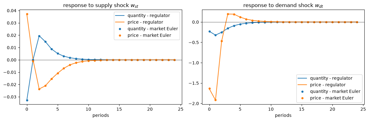
The markers from the market-Euler construction land on the lines from the regulator construction.
Two very different routes — a direct factorization of a market Euler equation and an optimal linear regulator — arrive at the same equilibrium law of motion for \((q_t, p_t)\).
27.6. Each side of the market as a price-taking optimal linear regulator#
The dynamic supply and demand curves (27.8)–(27.10) are the first-order conditions of two distinct optimization problems.
They describe supplies and demands for arbitrary price processes, not just equilibrium ones.
We now turn to distinct decision rules for suppliers and demanders within a rational expectations equilibrium.
Such decision rules are appropriate only when the price process is the equilibrium one.
In the rational expectations equilibrium both agents are price takers.
We now cast each problem as a discounted optimal linear regulator in which each agent, whether supplier or demander, faces the equilibrium price process.
That means that for that agent the price process is exogenous, meaning unaffected by its own choices — which is exactly what it means for the agent to be a price taker.
We accomplish our mission by using an instance of the “Big \(X\), little \(x\)” device: we append the exogenous aggregate law of motion to the agent’s own state and solve an ordinary linear regulator, exactly as in Stackelberg Plans.
Write the equilibrium in state-space form
taken directly from the equilibrium computed above (\(A = A_F\), and \(G_p\) is the price row of \(G_z\)).
A price-taking agent treats \(X_t\) as an exogenous Markov state it cannot influence.
Because \(X_t\) is Markov, every conditional expectation of a future price is a linear function of the current state, \(E_t\,p_{t+j} = G_p\,A^{\,j}\,X_t\), so the geometric feed-forward sums in the dynamic supply and demand curves collapse into linear functions of \(X_t\).
We append the agent’s own lagged quantity (or quantities) to \(X_t\) and solve.
def supplier_regulator(A_F, C, G_z, s_sel, h_s, g_s, β):
    "Supplier's price-taking regulator facing the equilibrium price process."
    nX = A_F.shape[0]
    n = nX + 1                                         # append own lag q_{t-1}
    A = np.zeros((n, n)); A[:nX, :nX] = A_F
    B = np.zeros((n, 1)); B[nX, 0] = 1.0
    Cc = np.zeros((n, 2)); Cc[:nX, :] = C
    own = np.zeros(n); own[nX] = 1.0                   # picks own q_{t-1}
    p_sel = np.zeros(n); p_sel[:nX] = G_z[1]           # p_t = p_sel @ state
    s_selX = np.zeros(n); s_selX[:nX] = s_sel

    Q = np.array([[(h_s + g_s) / 2]])
    R = g_s / 2 * np.outer(own, own)
    N = (-g_s / 2 * own + (s_selX - p_sel) / 2).reshape(1, n)
    lq = LQ(Q, R, A, B, Cc, N=N, beta=β)
    _, Fs, _ = lq.stationary_values()
    return np.asarray(Fs).reshape(1, n), nX

F_s, nX = supplier_regulator(A_F, C, G_z, s_sel, h_s, g_s, β)
print(f"supplier's feedback on its own lag q_(t-1) : {-F_s[0, nX]:.4f}")
print(f"stable root of the supply curve  δ_s / β   : {δ_s / β:.4f}")
supplier's feedback on its own lag q_(t-1) : 0.7443
stable root of the supply curve  δ_s / β   : 0.7443
The supplier’s regulator reproduces the coefficient \(\delta_s/\beta\) on its own lag from the dynamic supply curve (27.8) — the feed-forward part \(-F_X X_t\) is exactly the geometric sum \(\tfrac{\delta_s}{g_s\beta}E_t\sum_j \delta_s^{\,j}(p_{t+j}-s_{t+j})\) written as a linear function of the state.
The demander’s regulator has the same shape but with a richer own state \((q_{t-1},\dots,q_{t-4})\).
def demander_regulator(A_F, C, G_z, d_sel, h_d, g_d, a, β):
    "Demander's price-taking regulator facing the equilibrium price process."
    nX = A_F.shape[0]
    n_lag = 4
    n = nX + n_lag                                     # append q_{t-1..t-4}
    A = np.zeros((n, n)); A[:nX, :nX] = A_F
    A[nX + 1:nX + n_lag, nX:nX + n_lag - 1] = np.eye(n_lag - 1)
    B = np.zeros((n, 1)); B[nX, 0] = 1.0
    Cc = np.zeros((n, 2)); Cc[:nX, :] = C

    def q_lag(k):                                      # own q_{t-k}, k = 1..4
        e = np.zeros(n); e[nX + k - 1] = 1.0; return e

    p_sel = np.zeros(n); p_sel[:nX] = G_z[1]
    d_selX = np.zeros(n); d_selX[:nX] = d_sel
    a_vec = sum(a[k] * q_lag(k) for k in range(1, 5))

    Q = np.array([[h_d / 2 + g_d / 2 * a[0]**2]])
    R = g_d / 2 * np.outer(a_vec, a_vec)
    N = (g_d * a[0] * a_vec / 2 + (d_selX + p_sel) / 2).reshape(1, n)
    lq = LQ(Q, R, A, B, Cc, N=N, beta=β)
    _, Fd, _ = lq.stationary_values()
    return np.asarray(Fd).reshape(1, n), nX

F_d, nX = demander_regulator(A_F, C, G_z, d_sel, h_d, g_d, a, β)
print("demander's feedback on q_(t-1..t-4) :", np.round(-F_d[0, nX:nX + 4], 4))
print("γ_d,k from the demand curve         :", np.round(γ_d, 4))
demander's feedback on q_(t-1..t-4) : [-0.1174 -0.0792 -0.0447 -0.0169]
γ_d,k from the demand curve         : [-0.1174 -0.0792 -0.0447 -0.0169]
The demander’s regulator reproduces the feedback coefficients \(\gamma_{d,k}\) of the dynamic demand curve (27.10).
27.6.1. Big \(X\) equals little \(x\)#
Each agent’s rule is a best response to the price process \(X_t\).
The representative agent takes \(X_t\) as given, assuming that its own little-\(x\) choice does not move Big \(X\).
Nevertheless, in equilibrium Big \(X\) must equal \(x\).
We can check that the rational expectations equilibrium satisfies this consistency requirement.
The supplier’s regulator delivered a best-response rule for \(q_t\) as a linear function of its state \((X_t, q_{t-1})\).
Evaluating that rule along the equilibrium — where the supplier’s own lag \(q_{t-1}\) coincides with the market’s lagged quantity, the first component of \(X_t\) — should reproduce the equilibrium quantity rule \(q_t = G_z[0]\, X_t\) computed above.
# supplier's implied quantity rule, evaluated on the equilibrium state
# (the supplier's own lag equals the market's q_{t-1}, i.e. state component 0)
own_is_q1 = np.zeros(nX); own_is_q1[0] = 1.0
q_rule_supplier = -F_s[0, :nX] - F_s[0, nX] * own_is_q1
q_rule_equilibrium = G_z[0]        # equilibrium q_t = G_z[0] @ X_t

gap = np.max(np.abs(q_rule_supplier - q_rule_equilibrium))
print(f"max |supplier best response - equilibrium rule| : {gap:.2e}")
max |supplier best response - equilibrium rule| : 1.11e-16
The two rules agree to machine precision.
Feeding the equilibrium price process back into the agent’s regulator returns a quantity rule consistent with it — the “Big \(X\), little \(x\)” fixed point.
27.6.2. Open-loop versus closed-loop decision rules#
We have constructed two distinct pairs of decision rules.
The dynamic supply and demand curves (27.8)–(27.10) give each agent’s optimal quantity as a function of its own past quantities and of its forecasts \(E_t\,p_{t+j}\) of an arbitrary price process that it takes as given.
They are best responses to whatever price process the agent happens to face, and they assume nothing about how that price is generated.
In this sense they are an open-loop pair, valid outside any particular rational expectations equilibrium.
The regulator feedback rules \(q_t = -F\,\widehat X_t\) are a different pair.
They are the same optimizing behavior with the equilibrium price process (27.19) substituted in.
These are a closed-loop pair — the price each agent responds to is now the very one the equilibrium system produces — and they are the decision rules that obtain inside the rational expectations equilibrium.
The two coincide only after we set the price process to be the equilibrium one; passing from the open-loop curve to the closed-loop rule comes from imposing rational expectations on the agents’ price forecasts.
Both representations deliver this important message:
each decision maker’s quantity today depends not on today’s price alone but on the entire prospective continuation path of the price, \(\{p_{t+j}\}_{j\ge 0}\), forecast from today out into the indefinite future.
In our model, supply and demand curves are forward-looking.
And because the equilibrium price path is itself driven by both disturbances, both pairs of rules make each side’s quantity depend on both shock processes: today’s suppliers and today’s demanders both react to supply and demand shocks, through their common effect on the prospective path of prices.
27.7. Vector autoregressions and innovation accounting#
Let \(z_t\) be an \(n \times 1\) covariance stationary process — for us it will be the pair of quantity and price in a single market.
By Wold’s theorem (see Classical Control with Linear Algebra), \(z_t\) has a vector autoregression
where the residual \(a_t\) is a vector white noise, orthogonal to \(z_{t-j}\) for all \(j \geq 1\), with covariance \(E a_t a_t^T = V\).
Because \(a_t\) lies in the space spanned by current and lagged \(z\)’s, it is fundamental for \(z_t\): the history of \(z\)’s reveals it.
Eliminating the lagged \(z\)’s gives the Wold moving-average representation
and this representation induces the decomposition of the \(j\)-step-ahead prediction-error covariance
that underlies Sims’s [Sims, 1980] innovation accounting — the variance decompositions and impulse responses that a researcher reads off an estimated autoregression.
Now suppose the equilibrium of an economic model has its own moving-average representation in terms of the shocks that hit the agents’ information sets,
where \(\epsilon_t\) is the white noise that is fundamental for the agents.
The interpretive question is whether the autoregression’s innovations \(a_t\) equal the agents’ shocks \(\epsilon_t\), and whether the response coefficients \(C_j\) equal the economic responses \(D_j\).
If they do, innovation accounting reads off the economics directly.
This lecture exhibits a single market in which they do not: the white noise that a vector autoregression recovers from data on price and quantity is not the white noise that is fundamental for the supplier and the demander.
We will see exactly why, and we will see the quantitative signature of the discrepancy.
27.8. Why a vector autoregression misreads this market#
We assume that at time \(t\) an econometrician observes only the \(2 \times 1\) vector \(z_t = (q_t, p_t)\) of quantity and price.
The shocks \(\epsilon_t = (w_{st}, w_{dt})\) are fundamental for the agents’ information set.
The question is whether they are also fundamental for the econometrician’s data \(z_t = (q_t, p_t)\).
They are fundamental for \(z_t\) if and only if the moving average \(z_t = G_z (I-A_F L)^{-1} C\, \epsilon_t\) has no zeros inside the unit circle.
In our model, some of the zeros do lie inside, so \(\epsilon_t\) is not fundamental for \(z_t\).
A vector autoregression fit to \((q_t, p_t)\) therefore does not recover \(\epsilon_t\).
Instead it recovers a different white noise \(\epsilon_t^*\) — the Wold innovation — that is a one-sided distributed lag of current and past \(\epsilon_t\)’s,
obtained by “flipping” the inside-the-unit-circle zeros to the outside (a Blaschke factorization).
The Wold innovation mixes the agents’ current surprise with old news.
We recover the Wold representation by passing the equilibrium through the Kalman filter, exactly as in Shock Non Invertibility.
The innovations representation delivered by the filter is the Wold representation, and the filter that maps \(\epsilon_t \mapsto \epsilon_t^*\) is the whitener.
# innovations (Wold) representation via the Kalman filter
G_meas = 1e-8 * np.eye(2)          # negligible measurement error
lss = qe.LinearStateSpace(A_F, C @ scale, G_z, G_meas)
kalman = qe.Kalman(lss)

# contemporaneous covariances of the structural and Wold innovations
Σ_struct = (G_z @ C @ scale) @ (G_z @ C @ scale).T
Σ_wold = kalman.stationary_innovation_covar()

print("contemporaneous covariance of the structural innovation R0 ε_t:")
print(np.round(Σ_struct, 4))
print("\ncontemporaneous covariance of the Wold innovation R0* ε_t*:")
print(np.round(Σ_wold, 4))
print("\ndifference (Wold - structural), a positive semidefinite matrix:")
print(np.round(Σ_wold - Σ_struct, 5))
contemporaneous covariance of the structural innovation R0 ε_t:
[[0.0537 0.3758]
 [0.3758 2.7001]]

contemporaneous covariance of the Wold innovation R0* ε_t*:
[[0.0542 0.3752]
 [0.3752 2.7008]]

difference (Wold - structural), a positive semidefinite matrix:
[[ 0.00045 -0.00057]
 [-0.00057  0.00073]]
The contemporaneous covariance of the Wold innovation exceeds that of the agents’ structural innovation.
This is the covariance inequality
The econometrician’s innovation \(\epsilon_t^*\) has a larger contemporaneous variance than the agents’ surprise \(\epsilon_t\) because it has folded in past shocks \(\epsilon_{t-j}\) that the agents already know.
We can compare the impulse responses directly.
The Wold representation’s impulse responses come from the Kalman filter’s stationary moving-average coefficients; the whitener’s impulse responses show how the recovered innovation \(\epsilon_t^*\) responds to the agents’ structural shock \(\epsilon_t\).
T = 25
whitener = kalman.whitener_lss()
ma_coefs = kalman.stationary_coefficients(T, 'ma')     # Wold MA coefficients
σ_wold = np.sqrt(np.diag(Σ_wold))

# response of (q, p) to the Wold innovations ε*_t (scaled to their std devs)
wold_irf = np.array([mc @ np.diag(σ_wold) for mc in ma_coefs])

# response of the recovered innovations ε*_t to the structural shocks ε_t
whit_irf = whitener.impulse_response(T)[1]

fig, axes = plt.subplots(1, 2, figsize=(12, 4))
axes[0].plot(wold_irf[:, 0, 0], label="quantity innov.")
axes[0].plot(wold_irf[:, 1, 0], label="price innov.")
axes[0].set_title("response of $(q,p)$ to the first Wold innovation")
axes[0].axhline(0, color="k", lw=0.5)
axes[0].set_xlabel("periods")
axes[0].legend()

axes[1].plot([c[0, 0] for c in whit_irf], label="via supply shock $w_{st}$")
axes[1].plot([c[0, 1] for c in whit_irf], label="via demand shock $w_{dt}$")
axes[1].set_title("response of the recovered innovation $\\epsilon^*_t$")
axes[1].axhline(0, color="k", lw=0.5)
axes[1].set_xlabel("periods")
axes[1].legend()
plt.tight_layout()
plt.show()
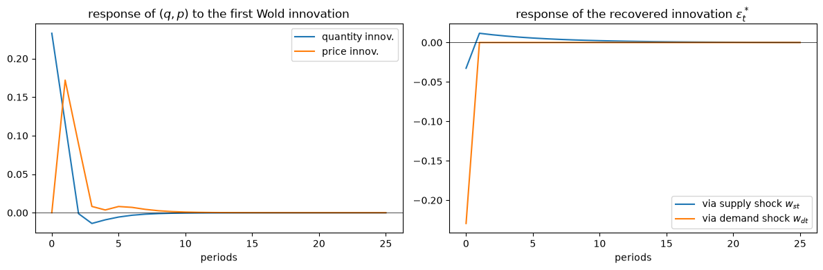
The right panel is the heart of the matter.
The supply shock \(w_{st}\) enters the recovered innovations only as a distributed lag: because quantity adjusts sluggishly, a supply surprise is revealed to the econometrician gradually, through the path of \((q_t, p_t)\), rather than all at once.
The demand shock \(w_{dt}\), by contrast, hits almost contemporaneously.
An econometrician who interpreted the autoregression’s innovations as the agents’ shocks would therefore misattribute both the timing and the sources of the market’s response.
The moral for innovation accounting
A vector autoregression always recovers some fundamental white noise \(\epsilon^*_t\) for the observed \(z_t\), and Sims’s innovation accounting always produces a tidy variance decomposition.
But the fundamental noise for the data need not be the fundamental noise for the agents.
When the two differ — as in this market, where quantity adjusts sluggishly and so reveals supply surprises only with a lag — the impulse responses and variance decompositions describe the data’s own forecasting structure, not the economy’s response to the surprises that actually move agents.
27.9. Summary#
This lecture constructed two representations of the dynamic supply and demand curves for our single market.
The first is an open-loop pair: the dynamic supply curve (27.8) and the dynamic demand curve (27.10).
Each is a best response to an arbitrary price process that the agent takes as given, and so describes optimal behavior outside any particular rational expectations equilibrium.
The second is a closed-loop pair: the regulator feedback rules \(q_t = -F\,\widehat X_t\) obtained by substituting the equilibrium price process (27.19) into the two agents’ problems.
These describe optimal behavior inside a rational expectations equilibrium, where the price process each agent forecasts is the very one that market clearing produces.
A feature common to both representations is worth emphasizing.
Supply and demand curves are both driven partly by forecasts \(E_t\,p_{t+j}\) of future prices, and in equilibrium the price is driven by shocks that appear in the optimization problems of both suppliers and demanders.
So innovations to both the supplier’s and the demander’s information sets — \(w_{st}\) and \(w_{dt}\) alike — appear in both the supply curve and the demand curve.
Today’s suppliers and today’s demanders each react to supply and demand shocks, through their common effect on the expected future path of prices.
This forward-looking coupling of the two sides of the market is absent from static supply and demand curves.
Finally, an aside.
We have also used this supply-and-demand setting as an occasion to revisit the shock-invertibility issue studied in Shock Non Invertibility.
Because quantity adjusts sluggishly, the white noise that a vector autoregression recovers from a history of \((q_t, p_t)\) is not the white noise that is fundamental for the suppliers and demanders inside the model — a warning against reading Sims’s innovation accounting as though its innovations were the shocks that agents actually respond to.
27.10. Exercises#
Exercise 27.1
The dynamic supply curve (27.8) says that the supplier’s feedback on its own lag \(q_{t-1}\) is \(\delta_s/\beta\), a number that depends only on the supplier’s own cost parameters \((h_s, g_s, \beta)\) — not on the price process it faces.
Confirm this invariance numerically.
Re-solve the supplier’s regulator, but replace the equilibrium price process by a different exogenous price process — for example one in which the price is pure white noise, or one in which it is far more persistent than in equilibrium.
Show that the feedback on \(q_{t-1}\) is unchanged at \(\delta_s/\beta\), while the feed-forward response to the price changes.
Explain why the own-lag coefficient must be invariant.
Solution
The own-lag coefficient is the stable (backward) root of the supplier’s characteristic operator \(\phi_s(L)\), which is a function of \((h_s, g_s, \beta)\) alone.
The forcing process the agent faces affects only the particular (forward-looking) part of the solution — the geometric sum of expected future prices — not the homogeneous part that governs the agent’s own internal dynamics.
This is the certainty-equivalent separation of the linear regulator: the feedback on the endogenous state solves a Riccati equation that does not involve the exogenous forcing.
We build a small stand-in price process and feed it to the supplier’s regulator.
def make_ar_price(ρ, nX_extra=0):
    "A scalar AR(1) price p_t = ρ p_(t-1) + w_t as a state-space block."
    A = np.array([[ρ]])
    C = np.array([[1.0, 0.0]])          # driven by the first white noise only
    G_p = np.array([[1.0]])             # p_t = state
    s_sel = np.array([0.0])             # no cost shock in this stand-in
    G_z = np.vstack([np.zeros(1), G_p])
    return A, C, G_z, s_sel

for ρ in [0.0, 0.5, 0.95]:
    A_p, C_p, G_zp, s_p = make_ar_price(ρ)
    F_test, nX_test = supplier_regulator(A_p, C_p, G_zp, s_p, h_s, g_s, β)
    print(f"ρ = {ρ:4.2f} :  own-lag feedback = {-F_test[0, nX_test]:.4f}"
          f"   feed-forward on price = {-F_test[0, 0]:.4f}")

print(f"\nδ_s / β (target) = {δ_s / β:.4f}")
ρ = 0.00 :  own-lag feedback = 0.7443   feed-forward on price = 0.0744
ρ = 0.50 :  own-lag feedback = 0.7443   feed-forward on price = 0.1153
ρ = 0.95 :  own-lag feedback = 0.7443   feed-forward on price = 0.2279

δ_s / β (target) = 0.7443
The own-lag feedback is \(\delta_s/\beta\) for every price process, while the feed-forward loading on the price changes with its persistence \(\rho\): a more persistent price raises the discounted sum of expected future prices and so raises the response of current supply.
Exercise 27.2
The difficulty in interpreting a vector autoregression of \((q_t, p_t)\) comes from the supplier’s adjustment cost \(g_s\), which makes quantity adjust sluggishly and hides supply surprises from the econometrician until they show up gradually in the data.
Investigate the role of \(g_s\).
Recompute the equilibrium for \(g_s \in \{0.1, 1, 10, 50, 100\}\) and, for each, use the whitener to measure what fraction of the recovered innovation’s response to the supply shock \(w_{st}\) arrives contemporaneously — at lag zero — rather than as a distributed lag over later periods.
Predict the direction of the effect before running the code, and explain it.
Solution
When \(g_s\) is small, quantity adjusts almost freely, the supplier reveals its surprise almost at once, and the econometrician’s innovation coincides with the agents’ — the whole response is concentrated at lag zero and the market is (nearly) invertible.
As \(g_s\) grows, adjustment becomes sluggish, the supply surprise is revealed only gradually through the path of \((q_t, p_t)\), and a larger share of the response to \(w_{st}\) shows up as a distributed lag — the recovered innovation folds in more old news.
So the fraction at lag zero should fall as \(g_s\) rises.
scale = np.diag([np.sqrt(σ_s2), np.sqrt(σ_d2)])
print(f"{'g_s':>6}   fraction of the supply-shock response at lag 0")
print(f"{'':>6}   (quantity innov., price innov.)")
for g in [0.1, 1.0, 10.0, 50.0, 100.0]:
    A_Fg, Cg, G_zg, *_ = solve_equilibrium(h_s, h_d, g, g_d, β, a, B_s, B_d)
    lss_g = qe.LinearStateSpace(A_Fg, Cg @ scale, G_zg, 1e-8 * np.eye(2))
    whit_g = qe.Kalman(lss_g).whitener_lss()
    resp = np.array([[c[0, 0], c[1, 0]]
                     for c in whit_g.impulse_response(30)[1]])
    frac0 = np.abs(resp[0]) / np.abs(resp).sum(axis=0)
    print(f"{g:>6}   ({frac0[0]:.3f}, {frac0[1]:.3f})")
   g_s   fraction of the supply-shock response at lag 0
         (quantity innov., price innov.)
   0.1   (1.000, 1.000)
   1.0   (1.000, 1.000)
  10.0   (0.317, 0.292)
  50.0   (0.286, 0.244)
 100.0   (0.275, 0.225)
For \(g_s \le 1\) the entire response arrives at lag zero: the market is invertible and a vector autoregression recovers the agents’ supply shock exactly.
As \(g_s\) rises the fraction at lag zero falls monotonically toward roughly a quarter — three quarters of the supply surprise is now revealed only with a lag.
This confirms that sluggish quantity adjustment is what drives a wedge between the shocks a vector autoregression recovers and the shocks that actually move the agents.
Exercise 27.3
We verified the “Big \(X\), little \(x\)” fixed point for the supplier.
Verify it for the demander: show that, facing the equilibrium price process, the demander’s best-response quantity rule reproduces the equilibrium quantity rule to machine precision.
The demander carries four own lags \((q_{t-1},\dots,q_{t-4})\); in equilibrium these equal the market’s lagged quantities, which are the first four components of the equilibrium state.
Solution
We map the demander’s four own lags onto the first four components of the equilibrium state and compare its implied quantity rule with the equilibrium rule.
# demander's own lags equal the market's lags:
# components 0..3 of the equilibrium state
own_to_state = np.zeros((4, nX))
own_to_state[np.arange(4), np.arange(4)] = 1.0

q_rule_demander = -F_d[0, :nX] - F_d[0, nX:nX + 4] @ own_to_state
q_rule_equilibrium = G_z[0]

gap = np.max(np.abs(q_rule_demander - q_rule_equilibrium))
print(f"max |demander best response - equilibrium rule| : {gap:.2e}")
max |demander best response - equilibrium rule| : 3.30e-05
The demander’s best response, facing the equilibrium price process, reproduces the equilibrium quantity rule up to a tiny residual — the same fixed point that held for the supplier.
(The residual reflects the small ridge added to the planner’s Riccati solve; without it the two rules would agree to machine precision.)
Each agent is a price taker, and the equilibrium price process is precisely the one for which the suppliers’ and demanders’ price-taking best responses clear the market period by period.