
28. Induced Priors for Impulse Responses#
28.1. Overview#
This lecture uses the market for a single good studied in Dynamic Supply and Demand Curves as a laboratory.
We imagine a structural modeler who believes that model and knows all of its parameters except two adjustment-cost parameters, the supplier’s \(g_s\) and the demander’s \(g_d\).
The modeler expresses uncertainty about \((g_s, g_d)\) with a Bayesian prior.
Because every object that the model implies — impulse responses, autocovariances, the vector autoregression that an econometrician would fit to prices and quantities — is a function of \((g_s, g_d)\), the prior on \((g_s, g_d)\) induces a prior over each of those objects.
We approximate these induced priors by Monte Carlo.
In this lecture, we shall
compute the induced prior over the impulse responses of price \(p_t\) and quantity \(q_t\) to the supply shock \(w_{st}\) and the demand shock \(w_{dt}\) that hit the agents’ information sets,
compute the induced prior over the autocovariance function of \((q_t, p_t)\) — everything that an infinitely long sample could reveal,
compute the induced prior over the population vector autoregression for \((q_t, p_t)\): the covariance matrix of its innovations and its impulse responses under two standard recursive (Cholesky) orthogonalizations, one that puts \(q_t\) first and one that puts \(p_t\) first,
compare the induced priors over the VAR impulse responses with those over the structural impulse responses,
use the induced prior to construct sign restrictions motivated by economic theory in the spirit of Uhlig [2005], Uhlig [2017], and then ask what those sign restrictions can and cannot recover from a VAR, and
widen the prior, and then change its shape from uniform to log-uniform, to see how the induced priors, the region in which the supply shock is fundamental, and the performance of sign restrictions change.
The last step brings us back to the shock-invertibility issue that occupied Dynamic Supply and Demand Curves and Shock Non Invertibility.
We shall see that sign restrictions that are true — they hold with prior probability one under the modeler’s theory — can nonetheless identify a set of VAR impulse responses that excludes the true response to a supply shock.
In addition to what’s in Anaconda, this lecture uses the quantecon library.
!pip install --upgrade quantecon
We’ll make these imports:
import numpy as np
import quantecon as qe
import matplotlib.pyplot as plt
from scipy.linalg import solve_discrete_lyapunov
28.2. Background: sign restrictions#
Uhlig [2005] proposed an “agnostic” way to identify shocks in a vector autoregression.
Let \(u_t\) be the one-step-ahead prediction error of a VAR, with covariance matrix \(V = \mathbb{E}[u_t u_t^\top]\).
A researcher wants to write \(u_t = A \epsilon_t\), where \(\epsilon_t\) is a vector of mutually uncorrelated, unit-variance structural shocks, so that \(V = A A^\top\).
The covariance matrix \(V\) does not pin down \(A\).
If \(L\) is the lower-triangular Cholesky factor of \(V\), every factorization takes the form
so that a column \(a\) of \(A\) — what Uhlig calls an impulse vector — satisfies \(a = L r\) for some vector \(r\) of unit length.
A Cholesky decomposition picks \(R = I\), and with it a recursive “causal ordering” of the variables.
Uhlig instead imposes inequality restrictions on the signs of impulse responses, for example that a contractionary monetary policy shock does not raise prices for \(K\) periods, and treats every rotation \(R\) that satisfies the restrictions as admissible.
Drawing \(r\) uniformly from the unit sphere (the Haar measure) and discarding draws that violate the restrictions gives a sample from a prior that is flat on the admissible set.
Uhlig [2017] illustrates the logic with a static supply-and-demand example in which “supply slopes up, demand slopes down” delivers the sign pattern
and he summarizes his advice with two principles: if you know it, impose it; if you do not know it, do not impose it.
Where do sign restrictions come from?
They are supposed to be implications of economic theory that are robust across the range of theories, or of parameter values, that an audience finds plausible.
An induced prior makes that idea precise: a sign that holds for every parameter vector in the support of the prior is an implication of the theory that a believer can impose with confidence.
28.3. The structural model and the prior#
The model is the one in Dynamic Supply and Demand Curves, which we briefly recall.
A representative supplier and a representative demander each solve a linear-quadratic problem, taking the price process as given.
The supplier faces adjustment costs \(\tfrac{g_s}{2}(q_t - q_{t-1})^2\) and a cost shock \(s_t = B_s(L) w_{st}\); the demander values durable services \(a(L) q_t\) with adjustment cost \(\tfrac{g_d}{2}(a(L)q_t)^2\) and faces a demand shock \(d_t = B_d(L) w_{dt}\).
The shocks \(w_{st}, w_{dt}\) are mutually uncorrelated white noises with variances \(\sigma_s^2 = 0.5\) and \(\sigma_d^2 = 4\).
The rational expectations equilibrium has the state-space representation
with \(\epsilon_t = (w_{st}, w_{dt})\).
The modeler knows
and the two shock variances.
The modeler does not know the adjustment-cost parameters.
Instead of the values \(g_s = 10\) and \(g_d = 0.1\) used in Dynamic Supply and Demand Curves, the modeler has independent uniform priors
We continue to call \((g_s, g_d) = (10, 0.1)\) the true parameter values.
h_s = h_d = 1.0
β = 1 / 1.05
a = np.array([1, .8, .6, .4, .2])       # a(L): coefficients a0..a4

# MA polynomials for the shocks (coefficients on L^0..L^3)
B_d = np.convolve(np.convolve([1, .6], [1, .4]), [1, .2])
B_s = np.convolve(np.convolve([1, -.8], [1, .4]), [1, .2])

σ_s2, σ_d2 = 0.5, 4.0                   # shock variances
scale = np.diag([np.sqrt(σ_s2), np.sqrt(σ_d2)])

g_s_true, g_d_true = 10.0, 0.1          # the "true" values
g_s_lo, g_s_hi = 8.0, 12.0              # prior support for g_s
g_d_lo, g_d_hi = 0.05, 0.15             # prior support for g_d
We solve for the equilibrium exactly as in Dynamic Supply and Demand Curves, as the optimal linear regulator of a fictitious planner.
def companion_shift(n):
    "Companion matrix that shifts an n-vector of lagged shocks."
    A = np.zeros((n, n))
    A[1:, :-1] = np.eye(n - 1)
    return A

def solve_equilibrium(h_s, h_d, g_s, g_d, β, a, B_s, B_d):
    """
    Solve the market equilibrium as a planner's optimal linear regulator.

    State x = [q_{t-1}, ..., q_{t-4}, w_s(t..t-3), w_d(t..t-3)]   (dim 12)
    Control u = q_t.

    Returns the closed-loop transition A_F, shock loading C, the selector
    G_z mapping the state into (q_t, p_t), and the selectors for s_t, d_t.
    """
    n_q = 4
    # exogenous companion for the two MA(3) shock processes
    A_w = np.zeros((8, 8))
    A_w[:4, :4] = companion_shift(4)
    A_w[4:, 4:] = companion_shift(4)
    C_w = np.zeros((8, 2))
    C_w[0, 0], C_w[4, 1] = 1.0, 1.0                    # inject (w_s, w_d)

    n = n_q + 8
    A = np.zeros((n, n))
    A[1:n_q, 0:n_q - 1] = np.eye(n_q - 1)              # q lags shift
    A[n_q:, n_q:] = A_w
    B = np.zeros((n, 1))
    B[0, 0] = 1.0                                      # new q_{t-1} = q_t
    C = np.zeros((n, 2))
    C[n_q:, :] = C_w

    def q_lag(k):                                      # selector for q_{t-k}
        e = np.zeros(n)
        e[k - 1] = 1.0
        return e

    s_sel = np.zeros(n)
    s_sel[n_q:n_q + 4] = B_s                           # s_t = s_sel @ x
    d_sel = np.zeros(n)
    d_sel[n_q + 4:] = B_d
    q1 = q_lag(1)
    a_vec = sum(a[k] * q_lag(k) for k in range(1, 5))  # lagged part of a(L)q_t

    # one-period loss = -(surplus), written as u'Qu + x'Rx + 2 u'Nx
    Q = np.array([[(h_s + h_d) / 2 + g_s / 2 + g_d / 2 * a[0]**2]])
    R = g_d / 2 * np.outer(a_vec, a_vec) + g_s / 2 * np.outer(q1, q1)
    R += 1e-5 * np.eye(n)          # tiny ridge for the Riccati solver
    N = (g_d * a[0] * a_vec / 2 - g_s * q1 / 2
         + (s_sel + d_sel) / 2).reshape(1, n)

    lq = qe.LQ(Q, R, A, B, C, N=N, beta=β)
    P, F, _ = lq.stationary_values()
    F = np.asarray(F).reshape(1, n)
    A_F = A - B @ F

    # price p_t = s_t + h_s q_t + g_s[(1+β) q_t - q_{t-1} - β E_t q_{t+1}]
    F_q = -F                                           # q_t = F_q @ x
    E_q1 = -F @ A_F                                    # E_t q_{t+1} = E_q1 @ x
    G_p = (s_sel + h_s * F_q[0] + g_s * (1 + β) * F_q[0]
           - g_s * q1 - g_s * β * E_q1[0]).reshape(1, n)
    G_z = np.vstack([F_q, G_p])                        # (q_t, p_t) = G_z @ x
    return A_F, C, G_z, F, s_sel, d_sel
28.3.1. A sign convention#
In Dynamic Supply and Demand Curves, a positive \(w_{st}\) raises the supplier’s costs and a positive \(w_{dt}\) lowers the demander’s willingness to pay, so both push quantity down.
To match the convention in [Uhlig, 2017] that a positive shock raises quantity, we work with
each scaled to one standard deviation.
From now on “the supply shock” and “the demand shock” refer to \(\tilde w_{st}\) and \(\tilde w_{dt}\).
28.4. Induced priors by Monte Carlo#
Let \(\theta = (g_s, g_d)\) have prior density \(\pi(\theta)\) and let \(f(\theta)\) be any object that the model implies, for example the impulse response of \(p_{t+j}\) to \(\tilde w_{dt}\).
The induced prior over \(f\) is the probability distribution of the random variable \(f(\theta)\) when \(\theta \sim \pi\).
It is the push-forward of \(\pi\) through the mapping \(f\).
Typically \(f\) is a complicated nonlinear function — here it requires solving a Riccati equation, and for the VAR objects a second Riccati equation for a Kalman filter — so we can’t write down the induced prior in closed form.
Monte Carlo is the natural tool:
draw \(\theta_i \sim \pi\) for \(i = 1, \ldots, N\),
compute \(f(\theta_i)\),
treat \(\{f(\theta_i)\}_{i=1}^N\) as a sample from the induced prior.
Geweke [2010] calls this prior predictive analysis.
Leeper et al. [2017] use it to compute the range of government-spending multipliers — ratios of discounted impulse responses — that alternative DSGE specifications can produce before they confront data.
For impulse response functions we summarize the sample by pointwise quantiles, horizon by horizon.
As Uhlig [2017] reminds us (his Principle 17), a band built this way describes a collection of marginal distributions, one for each horizon; the curve that joins the pointwise medians is generally not the impulse response for any single draw \(\theta_i\).
For each draw we compute four objects.
Structural impulse responses \(D_j = G_z A_F^{\,j} \tilde C\), where \(\tilde C = -C\, \mathrm{diag}(\sigma_s, \sigma_d)\) loads the sign-flipped, unit-standard-deviation shocks.
Autocovariances \(\Gamma_j = \mathbb{E}[z_{t+j} z_t^\top] = G_z A_F^{\,j} \Sigma_X G_z^\top\), where \(\Sigma_X = A_F \Sigma_X A_F^\top + \tilde C \tilde C^\top\) is the stationary covariance of the state.
The innovation covariance \(V = \mathbb{E}[a_t a_t^\top]\) of the population VAR for \(z_t\).
The Wold moving-average coefficients \(C_j\) of the population VAR, with \(C_0 = I\).
As in Dynamic Supply and Demand Curves, the last two come from the stationary Kalman filter, whose innovations representation is the Wold representation \(z_t = \sum_{j \ge 0} C_j a_{t-j}\).
T = 20      # number of horizons j = 0, ..., T-1

def model_objects(g_s, g_d, T=T):
    "Structural IRFs, autocovariances, and population VAR objects at (g_s, g_d)."
    A_F, C, G_z, *_ = solve_equilibrium(h_s, h_d, g_s, g_d, β, a, B_s, B_d)
    C_tilde = -C @ scale          # favorable supply shock, positive demand shock

    # structural impulse responses D_j = G_z A_F^j C_tilde
    D = np.empty((T, 2, 2))
    M = C_tilde.copy()
    for j in range(T):
        D[j] = G_z @ M
        M = A_F @ M

    # autocovariances Γ_j = E z_{t+j} z_t'
    Σ_X = solve_discrete_lyapunov(A_F, C_tilde @ C_tilde.T)
    Γ = np.empty((T, 2, 2))
    M = Σ_X.copy()
    for j in range(T):
        Γ[j] = G_z @ M @ G_z.T
        M = A_F @ M

    # Wold (innovations) representation from the stationary Kalman filter
    lss = qe.LinearStateSpace(A_F, C_tilde, G_z, 1e-8 * np.eye(2))
    kalman = qe.Kalman(lss)
    kalman.stationary_values()
    V = kalman.stationary_innovation_covar()
    C_wold = np.array(kalman.stationary_coefficients(T - 1, 'ma'))
    A_var = np.array(kalman.stationary_coefficients(T - 1, 'var'))

    return dict(D=D, Γ=Γ, V=V, C=C_wold, A_var=A_var)
We take \(N = 2{,}000\) draws from the prior and also record the objects at the true parameter values.
rng = np.random.default_rng(1234)
N = 2_000
g_s_draws = rng.uniform(g_s_lo, g_s_hi, N)
g_d_draws = rng.uniform(g_d_lo, g_d_hi, N)

draws = [model_objects(gs, gd) for gs, gd in zip(g_s_draws, g_d_draws)]
D_draws = np.array([d['D'] for d in draws])          # (N, T, 2, 2)
Γ_draws = np.array([d['Γ'] for d in draws])
V_draws = np.array([d['V'] for d in draws])          # (N, 2, 2)
C_draws = np.array([d['C'] for d in draws])          # (N, T, 2, 2)
A_var_draws = np.array([d['A_var'] for d in draws])

truth = model_objects(g_s_true, g_d_true)
In every array of impulse responses, entry [j, i, k] is the response at horizon j of variable i
(\(0 = q\), \(1 = p\)) to shock k.
We’ll use a helper that draws a band between the 5th and 95th percentiles together with the median.
def fan(ax, paths, color, label, x=None, alpha=0.25):
    "Plot the 5-95 percentile band and the median of paths (draws x horizons)."
    lo, med, hi = np.percentile(paths, [5, 50, 95], axis=0)
    x = np.arange(paths.shape[1]) if x is None else x
    ax.fill_between(x, lo, hi, color=color, alpha=alpha, lw=0)
    ax.plot(x, med, color=color, lw=2, label=label)

var_names = ["quantity $q$", "price $p$"]
shock_names = ["supply shock $\\tilde w_s$", "demand shock $\\tilde w_d$"]
var_short = ["q", "p"]
28.5. Object 1: structural impulse responses#
The first figure shows the induced prior over the responses of \((q_t, p_t)\) to the two structural shocks.
The dashed black lines are the responses at the true parameter values.
fig, axes = plt.subplots(2, 2, figsize=(12, 7))
for i in range(2):
    for k in range(2):
        ax = axes[i, k]
        fan(ax, D_draws[:, :, i, k], 'C0', 'induced prior: median, 5-95%')
        ax.plot(truth['D'][:, i, k], 'k--', lw=2, label='true parameters')
        ax.axhline(0, color='k', lw=0.5)
        ax.set_title(f"response of {var_names[i]} to {shock_names[k]}")
        ax.set_xlabel("periods")
axes[0, 0].legend()
plt.tight_layout()
plt.show()
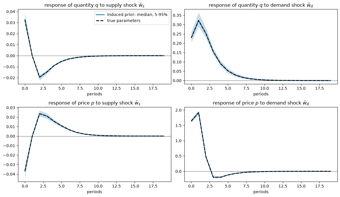
Fig. 28.1 Induced prior over structural impulse responses#
Over the ranges spanned by the prior, the qualitative shapes of the structural responses do not change.
A positive demand shock raises quantity for many periods and raises price for three periods, after which the price undershoots.
A favorable supply shock raises quantity and lowers price on impact, but its effects are small and change sign after a couple of periods — an imprint of the moving-average polynomial \(B_s(L) = 1 - .2L - .4L^2 - .064 L^3\), whose negative lag coefficients reverse the cost shock.
A uniform prior over a parameter generally induces a non-uniform prior over the responses.
The histograms below show the induced priors over the four impact responses.
fig, axes = plt.subplots(2, 2, figsize=(12, 6))
for i in range(2):
    for k in range(2):
        ax = axes[i, k]
        ax.hist(D_draws[:, 0, i, k], bins=40, density=True, color='C0', alpha=0.7)
        ax.axvline(truth['D'][0, i, k], color='k', ls='--')
        ax.set_title(f"impact response of {var_names[i]} to {shock_names[k]}")
plt.tight_layout()
plt.show()
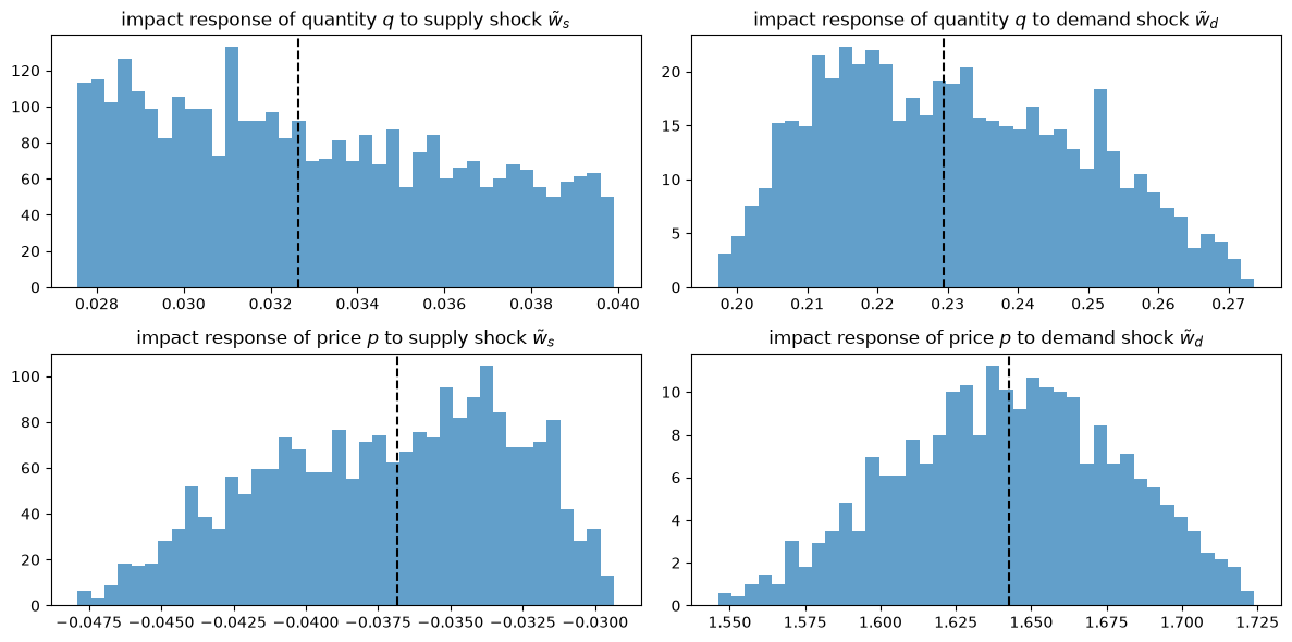
Fig. 28.2 Induced prior over impact responses#
Which uncertain parameter drives which response?
The correlations of the impact responses with the parameter draws tell us.
for i in range(2):
    for k in range(2):
        x = D_draws[:, 0, i, k]
        print(f"impact of {shock_names[k][:6]} on {var_short[i]}: "
              f"corr with g_s = {np.corrcoef(g_s_draws, x)[0, 1]:6.3f}, "
              f"corr with g_d = {np.corrcoef(g_d_draws, x)[0, 1]:6.3f}")
impact of supply on q: corr with g_s = -0.996, corr with g_d = -0.007
impact of demand on q: corr with g_s = -0.944, corr with g_d = -0.320
impact of supply on p: corr with g_s =  0.951, corr with g_d = -0.295
impact of demand on p: corr with g_s =  0.670, corr with g_d = -0.740
The response to the supply shock is governed almost entirely by the supplier’s adjustment cost \(g_s\): a larger \(g_s\) makes the supplier less willing to change output, so a given cost reduction moves quantity less.
The demander’s \(g_d\) matters mainly for the response of price to a demand shock.
28.5.1. The sign implications of the theory#
For each variable, shock, and horizon, we can compute the induced prior probability that the response is positive.
When that probability is one, the sign is an implication of the theory that is robust to the modeler’s uncertainty about \((g_s, g_d)\).
K_max = 5
prob_pos = (D_draws[:, :K_max + 1] > 0).mean(axis=0)     # (K_max+1, 2, 2)
prob_neg = (D_draws[:, :K_max + 1] < 0).mean(axis=0)

# +1: positive with prior probability one; -1: negative with probability one; 0: '?'
sign_table = np.where(prob_pos == 1, 1, np.where(prob_neg == 1, -1, 0))

symbol = {1: ' + ', -1: ' - ', 0: ' ? '}
print("horizon |  supply: q   p  |  demand: q   p")
for j in range(K_max + 1):
    s = [symbol[sign_table[j, i, k]] for k in range(2) for i in range(2)]
    print(f"   {j}    |     {s[0]}  {s[1]}   |     {s[2]}  {s[3]}")
horizon |  supply: q   p  |  demand: q   p
   0    |      +    -    |      +    +
   1    |      ?    ?    |      +    +
   2    |      -    +    |      +    +
   3    |      -    +    |      +    -
   4    |      -    +    |      +    -
   5    |      -    +    |      +    -
On impact, the theory delivers exactly the sign pattern in Uhlig’s static example: a favorable supply shock moves price and quantity in opposite directions, while a positive demand shock moves them in the same direction.
The theory says more than that.
It also signs most responses at longer horizons: the supply responses reverse sign from horizon 2 on, and the price response to a demand shock turns negative from horizon 3 on.
At horizon 1 the supply responses are almost exactly zero and their signs depend on \((g_s, g_d)\), so the theory is silent there.
print("prior probability that the horizon-1 supply responses are positive:")
print(f"  q: {prob_pos[1, 0, 0]:.3f},   p: {prob_pos[1, 1, 0]:.3f}")
prior probability that the horizon-1 supply responses are positive:
  q: 0.326,   p: 0.323
Leeper et al. [2017] report tables of exactly this kind — for example, the prior probability that a consumption multiplier is positive, horizon by horizon and model by model.
They put entries of 0 or 1 to the opposite use from Uhlig.
For Leeper, Traum, and Walker, such an entry is a warning that a model will deliver that sign no matter what the data say, so they prefer specifications whose induced priors leave signs open.
For Uhlig, the same entry is a restriction that the theory licenses and that is worth imposing.
28.6. Object 2: autocovariances#
An econometrician with an infinitely long sample of \((q_t, p_t)\) could learn the autocovariance function \(\{\Gamma_j\}\), and nothing more.
The induced prior over the autocovariance function is therefore the prior over everything that data could ever reveal.
We plot autocorrelations of \(q\) and \(p\) and the cross-correlation \(\mathrm{corr}(q_{t+j}, p_t)\), using \(\Gamma_{-j} = \Gamma_j^\top\) for negative \(j\).
sd = np.sqrt(np.stack([Γ_draws[:, 0, 0, 0], Γ_draws[:, 0, 1, 1]], axis=1))  # (N, 2)
ρ_q = Γ_draws[:, :, 0, 0] / sd[:, [0]]**2
ρ_p = Γ_draws[:, :, 1, 1] / sd[:, [1]]**2
# corr(q_{t+j}, p_t) for j >= 0 and corr(q_{t-j}, p_t) = corr(p_{t+j}, q_t) for j > 0
cross_pos = Γ_draws[:, :, 0, 1] / (sd[:, [0]] * sd[:, [1]])
cross_neg = Γ_draws[:, 1:, 1, 0] / (sd[:, [0]] * sd[:, [1]])
cross = np.hstack([cross_neg[:, ::-1], cross_pos])
lags = np.arange(-(T - 1), T)

fig, axes = plt.subplots(1, 3, figsize=(14, 4))
fan(axes[0], ρ_q, 'C0', 'induced prior')
axes[0].set_title("autocorrelation of $q$")
fan(axes[1], ρ_p, 'C1', 'induced prior')
axes[1].set_title("autocorrelation of $p$")
fan(axes[2], cross, 'C2', 'induced prior', x=lags)
axes[2].set_title("cross-correlation corr$(q_{t+j}, p_t)$")
for ax in axes:
    ax.axhline(0, color='k', lw=0.5)
    ax.set_xlabel("$j$")
plt.tight_layout()
plt.show()
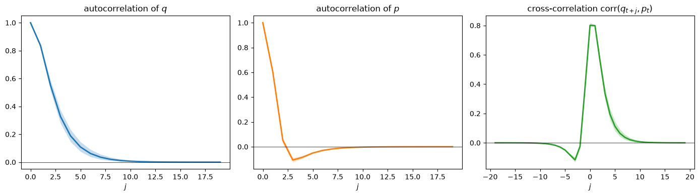
Fig. 28.3 Induced prior over correlations#
Quantity is much more persistent than price, an outcome of the large supply-side adjustment cost.
Quantity and price are strongly positively correlated contemporaneously, and price leads quantity.
28.7. Object 3: the population VAR#
By Wold’s theorem, \(z_t\) has a vector autoregression
with moving-average representation \(z_t = \sum_{j \ge 0} C_j a_{t-j}\), \(C_0 = I\).
The VAR coefficients \(A_j\), the innovation covariance \(V\), and the Wold coefficients \(C_j\) are all functions of the autocovariance function alone.
So the prior over \((g_s, g_d)\) also induces a prior over the reduced-form VAR, an idea that Del Negro and Schorfheide [2004] used to construct priors for VARs from equilibrium models.
The VAR has infinitely many lags, but its coefficients decay quickly.
size = np.abs(A_var_draws).max(axis=(2, 3))   # largest |entry| of A_j, lag by lag
fig, ax = plt.subplots()
fan(ax, np.log10(size), 'C0', 'induced prior', x=np.arange(1, T + 1))
ax.set_xlabel("lag $j$")
ax.set_ylabel("$\\log_{10} \\max |A_j|$")
plt.tight_layout()
plt.show()
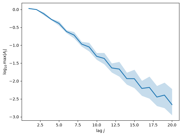
Fig. 28.4 Size of the VAR coefficients#
28.7.1. The innovation covariance matrix#
Next we look at the induced prior over the three distinct elements of \(V\), expressed as two standard deviations and a correlation.
sd_a = np.sqrt(np.stack([V_draws[:, 0, 0], V_draws[:, 1, 1]], axis=1))
corr_a = V_draws[:, 0, 1] / (sd_a[:, 0] * sd_a[:, 1])
V_true = truth['V']

fig, axes = plt.subplots(1, 3, figsize=(14, 3.5))
axes[0].hist(sd_a[:, 0], bins=40, density=True, color='C0', alpha=0.7)
axes[0].axvline(np.sqrt(V_true[0, 0]), color='k', ls='--')
axes[0].set_title("std. dev. of the $q$ innovation")
axes[1].hist(sd_a[:, 1], bins=40, density=True, color='C1', alpha=0.7)
axes[1].axvline(np.sqrt(V_true[1, 1]), color='k', ls='--')
axes[1].set_title("std. dev. of the $p$ innovation")
axes[2].hist(corr_a, bins=40, density=True, color='C2', alpha=0.7)
axes[2].axvline(V_true[0, 1] / np.sqrt(V_true[0, 0] * V_true[1, 1]),
                color='k', ls='--')
axes[2].set_title("correlation of the innovations")
plt.tight_layout()
plt.show()
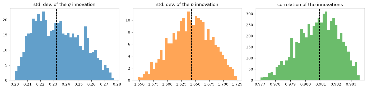
Fig. 28.5 Induced prior over innovation moments#
The innovations to quantity and price are almost perfectly correlated for every parameter value in the prior’s support.
print(f"range of corr(a_q, a_p) over the prior draws: "
      f"[{corr_a.min():.4f}, {corr_a.max():.4f}]")
range of corr(a_q, a_p) over the prior draws: [0.9770, 0.9836]
Demand shocks have a much larger variance than supply shocks and move \(q\) and \(p\) in the same direction, so they dominate the one-step-ahead prediction errors.
Uhlig [2017] shows that in a static market a nearly perfect positive price–quantity correlation is the case in which sign restrictions are most informative; we’ll return to that point below.
How does \(V\) compare with the covariance \(D_0 D_0^\top\) of the agents’ own one-step-ahead surprises \(D_0 \epsilon_t\)?
In Dynamic Supply and Demand Curves we saw that the econometrician’s innovations have the larger covariance, because the agents’ shocks are not fundamental for \((q_t, p_t)\).
Σ_struct = np.einsum('nij,nkj->nik', D_draws[:, 0], D_draws[:, 0])  # D_0 D_0'
gap = V_draws - Σ_struct
print("eigenvalues of V - D_0 D_0' are nonnegative in every draw:",
      np.all(np.linalg.eigvalsh(gap) > -1e-10))
for i, name in enumerate(["q", "p"]):
    rel = gap[:, i, i] / V_draws[:, i, i]
    print(f"(V - D_0 D_0')_{name}{name} / V_{name}{name}: "
          f"median {np.median(rel):.4f}, range [{rel.min():.4f}, {rel.max():.4f}]")
eigenvalues of V - D_0 D_0' are nonnegative in every draw: True
(V - D_0 D_0')_qq / V_qq: median 0.0083, range [0.0072, 0.0090]
(V - D_0 D_0')_pp / V_pp: median 0.0003, range [0.0002, 0.0004]
The gap is small relative to \(V\) — less than one percent of the variance of the quantity innovation.
But we’ll see that the gap is large relative to the contribution of the supply shock, and that is what matters for recovering the supply shock from a VAR.
28.7.2. Two Cholesky orthogonalizations#
The most common way to turn VAR innovations into “structural” shocks is a recursive orthogonalization.
\(q\) first. Factor \(V = L_q L_q^\top\) with \(L_q\) lower triangular. The first orthogonalized shock is the innovation in \(q_t\); the second is the part of the innovation in \(p_t\) orthogonal to it, and it does not move \(q_t\) on impact.
\(p\) first. Reorder the variables as \((p_t, q_t)\) and factor. The first shock is the innovation in \(p_t\); the second is the part of the innovation in \(q_t\) orthogonal to it, and it does not move \(p_t\) on impact.
In each case the impulse responses are \(C_j L\) for the corresponding impact matrix \(L\).
We normalize signs as Uhlig does, so that each shock raises quantity on impact; when a shock does not move quantity on impact, we normalize it so that it lowers price, as a favorable supply shock does.
P_swap = np.array([[0, 1], [1, 0]])

def normalize(A):
    "Flip columns so that q rises on impact, or, if q does not move, p falls."
    A = A.copy()
    for k in range(A.shape[1]):
        key = A[0, k] if abs(A[0, k]) > 1e-10 else -A[1, k]
        A[:, k] *= np.sign(key)
    return A

def cholesky_impact(V, first):
    "Impact matrix in (q, p) order; column 0 is the shock ordered first."
    if first == 'q':
        L = np.linalg.cholesky(V)
    else:
        L = P_swap @ np.linalg.cholesky(P_swap @ V @ P_swap)
    return normalize(L)

chol_irfs = {}
for first in ['q', 'p']:
    L_draws = np.array([cholesky_impact(V, first) for V in V_draws])
    chol_irfs[first] = np.einsum('ntij,njk->ntik', C_draws, L_draws)

chol_true = {first: truth['C'] @ cholesky_impact(truth['V'], first)
             for first in ['q', 'p']}
Because demand shocks dominate both innovations, the shock ordered first in either ordering is mostly a demand shock, and the shock ordered second is the natural candidate for a supply shock.
We therefore compare the first Cholesky shock with the demand shock and the second Cholesky shock with the supply shock.
def compare_plot(first):
    fig, axes = plt.subplots(2, 2, figsize=(12, 7))
    pairs = [(1, 0), (0, 1)]          # (structural shock, Cholesky shock)
    other = 'p' if first == 'q' else 'q'
    chol_names = [f"innovation in ${first}$ (ordered first)",
                  f"${other}$ innovation orthogonal to ${first}$ (ordered second)"]
    for col, (k_struct, k_chol) in enumerate(pairs):
        for i in range(2):
            ax = axes[i, col]
            fan(ax, D_draws[:, :, i, k_struct], 'gray',
                f"structural: {shock_names[k_struct]}")
            fan(ax, chol_irfs[first][:, :, i, k_chol], 'C3',
                f"VAR, {first} first: {chol_names[k_chol]}")
            ax.axhline(0, color='k', lw=0.5)
            ax.set_title(f"response of {var_names[i]}")
            ax.set_xlabel("periods")
        axes[0, col].legend(fontsize=8)
    plt.tight_layout()
    plt.show()
First the ordering that puts \(q_t\) first.
compare_plot('q')
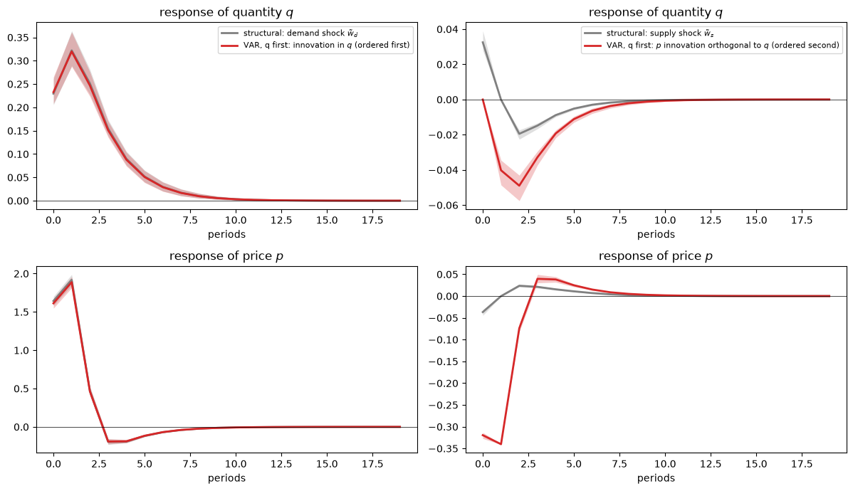
Fig. 28.6 Cholesky (\(q\) first) versus structural responses#
Then the ordering that puts \(p_t\) first.
compare_plot('p')
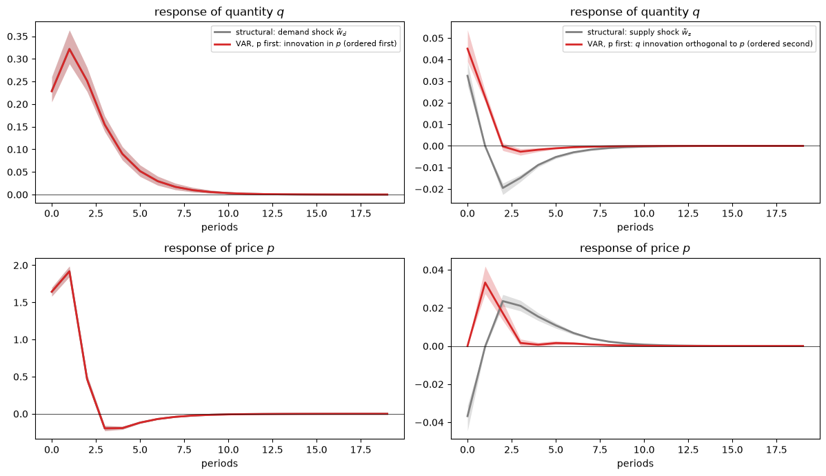
Fig. 28.7 Cholesky (\(p\) first) versus structural responses#
The left columns show that, in both orderings, the first Cholesky shock nearly reproduces the response to the demand shock.
The induced prior bands are almost indistinguishable — the \(p\)-first ordering does especially well, because the price innovation is almost entirely a demand surprise.
The right columns tell a different story.
Neither ordering produces anything that resembles the response to a supply shock.
With \(q\) first, the second shock does not move quantity on impact — by construction — while a supply shock raises it; the second shock lowers price on impact by roughly nine times as much as a supply shock does, and its quantity trough is about twice as deep.
With \(p\) first, the second shock does not move price on impact — again by construction — while a supply shock lowers it; the second shock overstates the impact on quantity, and its quantity response misses the sign reversal that the structural response displays from horizon 2 on.
These discrepancies hold for every parameter value in the prior’s support: both induced priors are concentrated, but they are concentrated in different places.
The numbers at the true parameters confirm this.
np.set_printoptions(precision=4, suppress=True)
print("impact responses (rows q, p) at the true parameters\n")
print("structural (supply, demand):\n", truth['D'][0])
print("\nq-first Cholesky (first, second):\n", chol_true['q'][0])
print("\np-first Cholesky (first, second):\n", chol_true['p'][0])
impact responses (rows q, p) at the true parameters

structural (supply, demand):
 [[ 0.0326  0.2295]
 [-0.0368  1.6428]]

q-first Cholesky (first, second):
 [[ 0.2328  0.    ]
 [ 1.612  -0.3196]]

p-first Cholesky (first, second):
 [[0.2283 0.0453]
 [1.6434 0.    ]]
28.8. Can any rotation recover the structural shocks?#
A Cholesky factorization is just one rotation.
Could some rotation \(R\) of the VAR innovations recover the structural impulse responses?
Uhlig’s Proposition A.1 [Uhlig, 2005] says that a vector \(d \in \mathbb{R}^2\) is an impulse vector of the VAR — a column of some \(A\) with \(A A^\top = V\) — if and only if \(d = L r\) with \(\|r\| = 1\), that is, if and only if
So we can ask, draw by draw, whether the structural impact vectors — the columns \(d_s, d_d\) of \(D_0\) — are admissible impulse vectors.
L_q_draws = np.linalg.cholesky(V_draws)
norms = np.linalg.norm(np.linalg.solve(L_q_draws, D_draws[:, 0]), axis=1)  # (N, 2)

fig, axes = plt.subplots(1, 2, figsize=(12, 3.5))
for k, ax in enumerate(axes):
    ax.hist(norms[:, k], bins=40, density=True, color=f'C{k}', alpha=0.7)
    ax.set_title(f"$\\|L^{{-1}} d\\|$ for the {shock_names[k]}")
plt.tight_layout()
plt.show()

for k in range(2):
    print(f"{shock_names[k][:6]}: ||L^-1 d|| in "
          f"[{norms[:, k].min():.4f}, {norms[:, k].max():.4f}]")
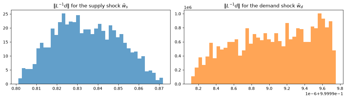
Fig. 28.8 Induced prior over \(\|L^{-1} d\|\)#
supply: ||L^-1 d|| in [0.8011, 0.8719]
demand: ||L^-1 d|| in [1.0000, 1.0000]
For the demand shock the norm is one, up to the accuracy of our computations: the demand shock is (almost) fundamental for \((q_t, p_t)\), and a suitable rotation of the VAR innovations recovers it.
For the supply shock the norm lies between \(0.80\) and \(0.87\) throughout the support of the prior.
No rotation of the VAR innovations can deliver the structural supply impact vector, because that vector is “too short”.
The reason is the one identified in Dynamic Supply and Demand Curves: because quantity adjusts sluggishly, a supply surprise is revealed to an econometrician only gradually, so the one-step-ahead VAR innovation contains only part of it, mixed with old news.
The structural moving average \(z_t = \sum_j D_j \epsilon_{t-j}\) and the Wold moving average \(z_t = \sum_j C_j a_{t-j}\) imply the same autocovariances, but \(\{D_j\}\) is not of the form \(\{C_j L R\}\) for any orthogonal \(R\).
28.9. Sign restrictions motivated by theory#
Now consider a second econometrician who has an infinite sample from the economy at the true parameter values, and so knows \(V\) and \(\{C_j\}\) exactly.
This econometrician is not willing to impose the whole structural model, but accepts the sign restrictions that the theory delivers with prior probability one — the table that we computed above.
Following Uhlig’s Principles 1 and 2, the econometrician imposes what is known and nothing more.
The econometrician applies Uhlig’s draw-and-reject algorithm:
draw \(r\) uniformly from the unit circle and form the orthogonal matrix \(R = [\,r,\ r^\perp\,]\), where \(r^\perp\) is \(r\) rotated by ninety degrees;
compute the impact matrix \(A = L R\), flipping the sign of each column so that quantity rises on impact, and the impulse responses \(C_j A\), treating the first column as the supply shock and the second as the demand shock;
keep the draw if the responses satisfy every restriction in the table at horizons \(j = 0, \ldots, K\);
repeat many times.
Because \(r\) ranges over the whole circle and signs are normalized afterwards, this procedure visits every orthogonal \(R\), including those that swap the roles of the two columns.
Because the likelihood is flat over the admissible rotations in an infinite sample, the kept draws form both the identified set and, with the Haar prior, the econometrician’s posterior (Uhlig’s Principle 9).
def sign_identified(C, V, table, K, n_draws=20_000, seed=0):
    """
    Uhlig's draw-and-reject algorithm.

    Returns the impulse responses (draws, T, 2, 2) of the kept rotations,
    with shock 0 = supply and shock 1 = demand, and the acceptance rate.
    """
    rng = np.random.default_rng(seed)
    L = np.linalg.cholesky(V)
    x = rng.standard_normal((n_draws, 2))
    r = x / np.linalg.norm(x, axis=1, keepdims=True)      # uniform on the circle
    R = np.stack([np.stack([r[:, 0], r[:, 1]], 1),
                  np.stack([-r[:, 1], r[:, 0]], 1)], axis=2)  # columns r, r_perp
    A = L @ R
    A = A * np.sign(A[:, [0], :])                           # q rises on impact
    irf = np.einsum('tij,njk->ntik', C, A)                  # (n_draws, T, 2, 2)

    ok = np.all(irf[:, :K + 1] * table[:K + 1] >= 0, axis=(1, 2, 3))
    return irf[ok], ok.mean()
We impose the restrictions on impact only (\(K = 0\)) and for six periods (\(K = 5\)).
sets = {}
for K in [0, K_max]:
    sets[K], acc = sign_identified(truth['C'], truth['V'], sign_table, K)
    print(f"K = {K}: acceptance rate {acc:.4f}")
K = 0: acceptance rate 0.0625
K = 5: acceptance rate 0.0122
Most draws are rejected.
That is good news, not bad: as Uhlig’s Principle 7 puts it, when a lot of draws are rejected, identification is sharp.
We plot the identified sets as the range between the smallest and largest response at each horizon, as in Figure 2 of Uhlig [2005], and compare them with the true structural responses and the \(p\)-first Cholesky responses.
fig, axes = plt.subplots(2, 2, figsize=(12, 7))
p_first_pair = {0: 1, 1: 0}   # structural shock -> p-first Cholesky column
for k in range(2):
    for i in range(2):
        ax = axes[i, k]
        for K, color in [(0, 'C0'), (K_max, 'C3')]:
            s = sets[K][:, :, i, k]
            ax.fill_between(range(T), s.min(0), s.max(0), color=color,
                            alpha=0.3, lw=0, label=f"sign-identified set, K = {K}")
        ax.plot(truth['D'][:, i, k], 'k--', lw=2, label='true structural response')
        ax.plot(chol_true['p'][:, i, p_first_pair[k]], 'C2', lw=2,
                label='p-first Cholesky')
        ax.axhline(0, color='k', lw=0.5)
        ax.set_title(f"response of {var_names[i]} to {shock_names[k]}")
        ax.set_xlabel("periods")
        ax.set_xlim(0, 12)
axes[0, 0].legend(fontsize=8)
plt.tight_layout()
plt.show()
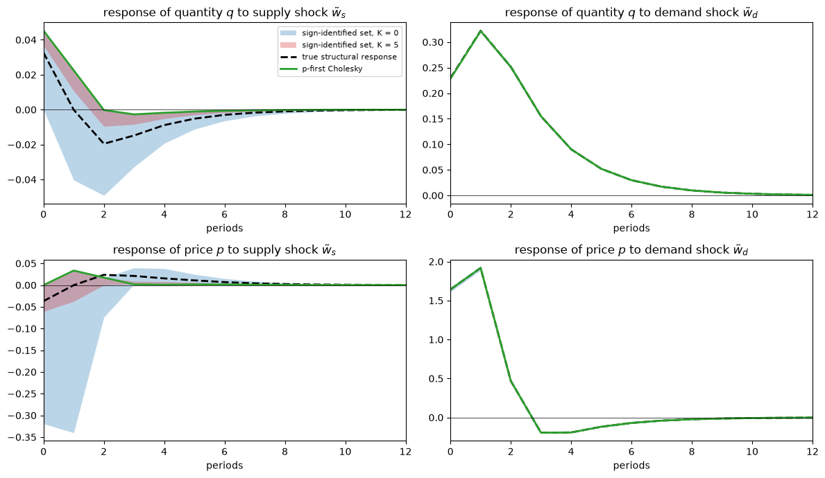
Fig. 28.9 Sign-identified sets at the true parameters#
The demand shock is identified almost exactly.
As Uhlig’s analysis of a static market predicts, the near-perfect positive correlation of the price and quantity innovations leaves very few rotations that move price and quantity in opposite directions for one shock and in the same direction for the other.
The supply shock is a different matter.
With restrictions on impact only, the identified set is wide: on impact the price response can be anywhere from zero to almost nine times its true value.
Imposing the restrictions for \(K = 5\) periods — restrictions that are correct, since the theory implies them for every parameter value in the prior’s support — narrows the set dramatically.
But the narrower set excludes the true response: the true response of quantity lies outside it at every horizon, and the true response of price from horizon 2 on.
One edge of the \(K = 5\) set is the \(p\)-first Cholesky response, which satisfies the restriction on the impact response of price only weakly, with a response of exactly zero.
s5 = sets[K_max][:, :, :, 0]
inside = ((s5.min(0) <= truth['D'][:, :, 0] + 1e-12)
          & (truth['D'][:, :, 0] <= s5.max(0) + 1e-12))
print("is the true supply response inside the K = 5 set?")
print("horizon:  ", np.arange(8))
print("quantity: ", inside[:8, 0])
print("price:    ", inside[:8, 1])
is the true supply response inside the K = 5 set?
horizon:   [0 1 2 3 4 5 6 7]
quantity:  [False False False False False False False False]
price:     [ True  True False False False False False False]
The explanation is the non-fundamentalness that we diagnosed above.
The sign restrictions are true statements about the structural responses \(D_j\).
But the econometrician can only search over responses of the form \(C_j L r\), and the true supply response is not among them.
The sign restrictions pick out the rotations that best mimic the signs of a supply shock, and those rotations get the magnitudes wrong.
Sign restrictions are a way to deal with an identification problem within the set of rotations of the VAR innovations; they offer no protection against the possibility that the shocks of interest are not rotations of the VAR innovations at all.
Uhlig [2017] explicitly sets aside “the thorny issue of fundamentalness”; our market shows why it deserves attention.
Information from outside the VAR can do what rotations cannot.
Policy Counterfactuals from Impulse Responses shows that a local projection on a noisy measure of the supply shock recovers the true supply-shock response, and that a sufficiently aggressive price-stabilizing tax rule makes the supply shock fundamental, so that the same sign restrictions then succeed.
28.9.1. Robustness across the prior#
Is the exclusion of the truth special to \((g_s, g_d) = (10, 0.1)\)?
We repeat the exercise for a few hundred draws from the prior, treating each in turn as the truth, and record whether the true impact response of quantity to a supply shock lies in the \(K = 5\) identified set.
n_check = 300
covered = np.empty(n_check, dtype=bool)
for n in range(n_check):
    kept, _ = sign_identified(C_draws[n], V_draws[n], sign_table, K_max,
                              n_draws=5_000, seed=n)
    lo, hi = kept[:, 0, 0, 0].min(), kept[:, 0, 0, 0].max()
    covered[n] = lo <= D_draws[n, 0, 0, 0] <= hi
print(f"fraction of draws in which the K = {K_max} set contains the true "
      f"impact response of q to a supply shock: {covered.mean():.3f}")
fraction of draws in which the K = 5 set contains the true impact response of q to a supply shock: 0.007
Throughout the support of the prior, the theory-motivated sign restrictions identify a set that misses the true response.
28.10. Widening the prior#
So far the modeler has been fairly confident: \(g_s\) is known to within \(\pm 20\) percent and \(g_d\) to within \(\pm 50\) percent.
What happens to the induced priors when the modeler is less sure?
We compare the baseline prior with two wider uniform priors.
priors = {
    'baseline': ((g_s_lo, g_s_hi), (g_d_lo, g_d_hi)),
    'wider':    ((4.0, 20.0), (0.02, 0.3)),
    'widest':   ((1.5, 40.0), (0.005, 1.0)),
}

N_wide = 1_500
wide = {'baseline': dict(g_s=g_s_draws, g_d=g_d_draws,
                         D=D_draws, V=V_draws, C=C_draws)}
for name in ['wider', 'widest']:
    (gs_lo, gs_hi), (gd_lo, gd_hi) = priors[name]
    rng_w = np.random.default_rng(2024)
    gs = rng_w.uniform(gs_lo, gs_hi, N_wide)
    gd = rng_w.uniform(gd_lo, gd_hi, N_wide)
    objs = [model_objects(x, y) for x, y in zip(gs, gd)]
    wide[name] = dict(g_s=gs, g_d=gd,
                      D=np.array([o['D'] for o in objs]),
                      V=np.array([o['V'] for o in objs]),
                      C=np.array([o['C'] for o in objs]))
28.10.1. Bigger induced priors#
The figure overlays the three induced priors over the structural impulse responses.
colors = {'baseline': 'C0', 'wider': 'C1', 'widest': 'C3'}

fig, axes = plt.subplots(2, 2, figsize=(12, 7))
for name in ['widest', 'wider', 'baseline']:
    (gs_lo, gs_hi), (gd_lo, gd_hi) = priors[name]
    label = f"$g_s \\sim U[{gs_lo:g}, {gs_hi:g}]$, $g_d \\sim U[{gd_lo:g}, {gd_hi:g}]$"
    for i in range(2):
        for k in range(2):
            fan(axes[i, k], wide[name]['D'][:, :, i, k], colors[name], label,
                alpha=0.35)
for i in range(2):
    for k in range(2):
        axes[i, k].axhline(0, color='k', lw=0.5)
        axes[i, k].set_title(f"response of {var_names[i]} to {shock_names[k]}")
        axes[i, k].set_xlabel("periods")
        axes[i, k].set_xlim(0, 12)
axes[0, 0].legend(fontsize=8)
plt.tight_layout()
plt.show()
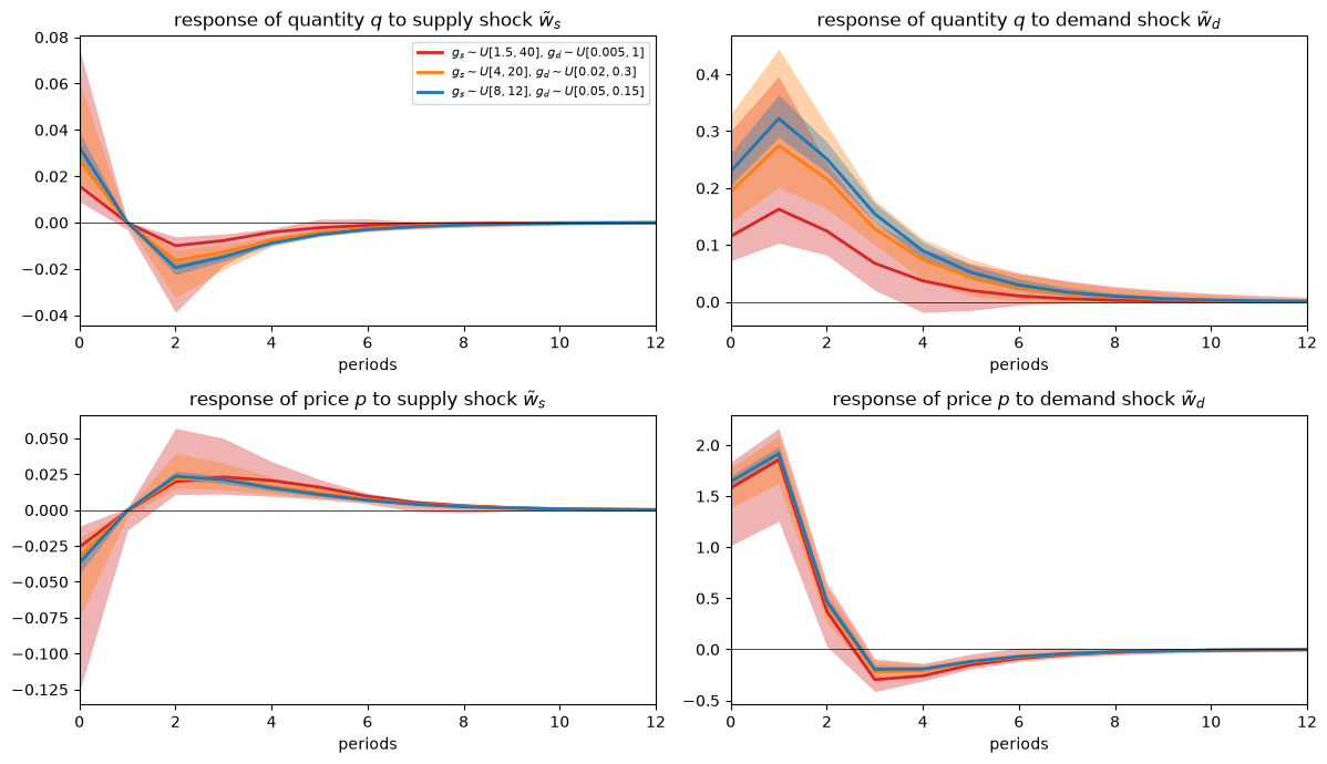
Fig. 28.10 Induced priors under wider priors#
The bands fan out as the prior widens, most of all for the impact responses to a supply shock and for the response of quantity to a demand shock.
Two features are worth noticing.
First, the induced prior moves as well as spreads: under the widest prior the median response of quantity to a demand shock is far below the baseline median.
A uniform prior on \([1.5, 40]\) puts most of its mass on large values of \(g_s\), at which suppliers adjust output very slowly, so “uniform” is far from “uninformative” about impulse responses (we return to this point below).
Second, some signs become uncertain: under the widest prior the response of quantity to a demand shock can turn negative after a few periods.
To see how the parameters map into responses, we plot the impact responses for each draw from the widest prior, coloring each point by its value of \(g_s\).
D_w, gs_w, gd_w = wide['widest']['D'], wide['widest']['g_s'], wide['widest']['g_d']

fig, axes = plt.subplots(1, 2, figsize=(12, 4.5))
for k, ax in enumerate(axes):
    sc = ax.scatter(D_w[:, 0, 0, k], D_w[:, 0, 1, k], c=gs_w, s=6, cmap='plasma')
    ax.set_xlabel("impact response of $q$")
    ax.set_ylabel("impact response of $p$")
    ax.set_title(f"impact responses to the {shock_names[k]}")
fig.colorbar(sc, ax=axes, label="$g_s$")
plt.show()
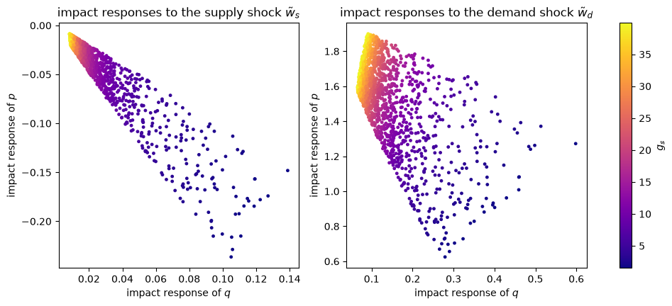
Fig. 28.11 Impact responses under the widest prior#
Each point is one economy.
A larger supply-side adjustment cost \(g_s\) shrinks the quantity response to both shocks, and the uniform prior’s concentration on large \(g_s\) piles the draws up in the upper-left corner of each cloud.
28.10.2. Where the supply shock is fundamental#
The same draws let us map where the supply shock can be recovered from a VAR.
We plot \(\|L^{-1} d_s\|\) against \(g_s\) and color each point by \(g_d\).
V_w = wide['widest']['V']
norms_w = np.linalg.norm(np.linalg.solve(np.linalg.cholesky(V_w), D_w[:, 0]), axis=1)

fig, ax = plt.subplots()
sc = ax.scatter(gs_w, norms_w[:, 0], c=gd_w, s=6, cmap='viridis')
ax.axhline(1, color='k', lw=0.5)
ax.set_xlabel("$g_s$")
ax.set_ylabel("$\\|L^{-1} d_s\\|$")
fig.colorbar(sc, ax=ax, label="$g_d$")
plt.tight_layout()
plt.show()
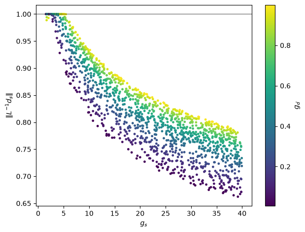
Fig. 28.12 Where the supply shock is fundamental#
For small \(g_s\), \(\|L^{-1} d_s\| = 1\): quantity adjusts quickly enough that a VAR innovation reveals the supply surprise at once, and the supply shock is fundamental for \((q_t, p_t)\).
Beyond a threshold that rises with \(g_d\), the norm falls below one and keeps falling as \(g_s\) grows.
The baseline prior \(g_s \in [8, 12]\) sits well inside the non-fundamental region.
28.10.3. What sign restrictions deliver under a wider prior#
A wider prior has a cost for the sign-restriction approach: fewer signs hold for every parameter value, so the theory licenses fewer restrictions.
def theory_signs(D, K=K_max):
    "Signs that hold with prior probability one: +1, -1, or 0 for '?'."
    pos = (D[:, :K + 1] > 0).mean(axis=0)
    neg = (D[:, :K + 1] < 0).mean(axis=0)
    return np.where(pos == 1, 1, np.where(neg == 1, -1, 0))

table_w = theory_signs(D_w)
print("signs implied by the widest prior")
print("horizon |  supply: q   p  |  demand: q   p")
for j in range(K_max + 1):
    s = [symbol[table_w[j, i, k]] for k in range(2) for i in range(2)]
    print(f"   {j}    |     {s[0]}  {s[1]}   |     {s[2]}  {s[3]}")
signs implied by the widest prior
horizon |  supply: q   p  |  demand: q   p
   0    |      +    -    |      +    +
   1    |      ?    ?    |      +    +
   2    |      -    +    |      +    ?
   3    |      -    +    |      ?    -
   4    |      ?    +    |      ?    -
   5    |      ?    +    |      ?    ?
Compared with the baseline table, several entries have become “?”.
Among the restrictions that survive is that a favorable supply shock raises price two periods later, the reversal that the cost-shock process \(B_s(L)\) builds in.
We now treat each draw from the widest prior in turn as the truth, give the econometrician its population VAR, impose the table above for \(K = 5\), and record one of three outcomes:
the sign-identified set contains the true impact response of quantity to a supply shock,
the set is nonempty but misses it, or
no rotation satisfies the restrictions at all.
def classify(C, V, D, table, K=K_max):
    """
    For each economy: 0 if no rotation is admissible, 1 if the identified set
    misses the true impact response of q to a supply shock, 2 if it contains it.
    """
    out = np.empty(len(D), dtype=int)
    for n in range(len(D)):
        kept, _ = sign_identified(C[n], V[n], table, K, n_draws=10_000, seed=n)
        if len(kept) == 0:
            out[n] = 0
        else:
            lo, hi = kept[:, 0, 0, 0].min(), kept[:, 0, 0, 0].max()
            out[n] = 2 if lo <= D[n, 0, 0, 0] <= hi else 1
    return out

outcome_labels = ["no admissible rotation", "set misses the truth",
                  "set contains the truth"]
outcome_colors = ['C7', 'C3', 'C2']

def outcome_map(ax, g_s, g_d, outcome, title=None):
    for code in range(3):
        m = outcome == code
        ax.scatter(g_s[m], g_d[m], s=8, color=outcome_colors[code],
                   label=f"{outcome_labels[code]} ({m.mean():.0%})")
    ax.set_xlabel("$g_s$")
    ax.set_ylabel("$g_d$")
    if title is not None:
        ax.set_title(title)
    ax.legend(loc='upper right', fontsize=9)

C_w = wide['widest']['C']
outcome = classify(C_w, V_w, D_w, table_w)

fig, ax = plt.subplots()
outcome_map(ax, gs_w, gd_w, outcome)
plt.tight_layout()
plt.show()
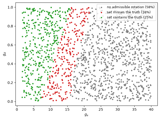
Fig. 28.13 Sign-restriction outcomes, uniform prior#
The parameter space splits into three regions.
For small \(g_s\) (green), the restrictions work as intended: the identified set contains the truth. This region includes the one where the supply shock is fundamental, and extends somewhat beyond it because the widest prior licenses fewer restrictions, which leaves wider identified sets.
For intermediate \(g_s\) (red), the set is nonempty but, as at our baseline parameters, it misses the truth.
For large \(g_s\) (gray), no rotation of the VAR innovations satisfies the restrictions.
In the gray region, an econometrician who applies Uhlig’s procedure to the population VAR finds that the sign restrictions are inconsistent with the data and would reject the theory that implied them — even though every restriction is a true statement about how the economy responds to its shocks.
Which restriction cannot be met?
We drop the horizon-2 restriction on the price response to a supply shock and try again on the gray draws.
table_drop = table_w.copy()
table_drop[2, 1, 0] = 0                   # horizon 2, price, supply shock
gray = np.where(outcome == 0)[0]
nonempty = [len(sign_identified(C_w[n], V_w[n], table_drop, K_max,
                                n_draws=10_000, seed=n)[0]) > 0 for n in gray]
print(f"gray draws with a nonempty set after dropping that restriction: "
      f"{np.mean(nonempty):.0%}")
gray draws with a nonempty set after dropping that restriction: 100%
The culprit is the delayed rise in price after a favorable supply shock.
When suppliers adjust slowly, the VAR innovations reveal that part of the supply shock’s propagation only gradually, so no rotation of them can reproduce it while also matching the signs on impact.
The lesson is that a broader prior can’t rescue the sign-restriction approach here.
Fewer restrictions survive, and for a large part of the prior’s support the restrictions that survive either miss the truth or cannot be satisfied at all.
28.10.4. A log-uniform prior on \(g_s\)#
The widest prior spans more than an order of magnitude, \(g_s \in [1.5, 40]\).
For a parameter like this — a positive scale parameter whose plausible values range over several multiples — a uniform prior is a strong opinion: it puts 65 percent of its mass on \([15, 40]\) and less than 7 percent on \([1.5, 4]\), even though each interval spans the same proportional range, a factor of \(8/3\).
A natural alternative is a log-uniform prior, under which \(\log g_s\) is uniform on \([\log 1.5, \log 40]\), so that every doubling of \(g_s\) receives the same prior probability.
Its density is proportional to \(1/g_s\) on the support.
We keep the uniform prior on \(g_d\) and the same supports, and change only the shape of the prior on \(g_s\).
(gs_lo, gs_hi), (gd_lo, gd_hi) = priors['widest']
rng_log = np.random.default_rng(2024)
gs_log = np.exp(rng_log.uniform(np.log(gs_lo), np.log(gs_hi), N_wide))
gd_log = rng_log.uniform(gd_lo, gd_hi, N_wide)
objs = [model_objects(x, y) for x, y in zip(gs_log, gd_log)]
wide['log-uniform'] = dict(g_s=gs_log, g_d=gd_log,
                           D=np.array([o['D'] for o in objs]),
                           V=np.array([o['V'] for o in objs]),
                           C=np.array([o['C'] for o in objs]))

gs_ticks = [2, 5, 10, 20, 40]

fig, ax = plt.subplots()
bins = np.geomspace(gs_lo, gs_hi, 30)                 # equally spaced in log g_s
w = np.full(N_wide, 1 / N_wide)
ax.hist(gs_w, bins=bins, weights=w, alpha=0.5, color='C3', label='uniform')
ax.hist(gs_log, bins=bins, weights=w, alpha=0.5, color='C4', label='log-uniform')
ax.set_xscale('log')
ax.set_xticks(gs_ticks, labels=[str(t) for t in gs_ticks])
ax.set_xlabel("$g_s$ (log scale)")
ax.set_ylabel("fraction of draws")
ax.legend()
plt.tight_layout()
plt.show()

for name, gs in [('uniform', gs_w), ('log-uniform', gs_log)]:
    print(f"{name:12s}: median g_s = {np.median(gs):5.2f},  "
          f"P(g_s < 4) = {np.mean(gs < 4):.2f},  P(g_s > 15) = {np.mean(gs > 15):.2f}")
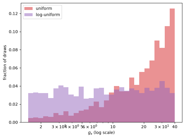
Fig. 28.14 Draws of \(g_s\) under two priors#
uniform     : median g_s = 21.47,  P(g_s < 4) = 0.06,  P(g_s > 15) = 0.66
log-uniform : median g_s =  8.24,  P(g_s < 4) = 0.29,  P(g_s > 15) = 0.31
On a logarithmic axis the log-uniform draws are spread evenly, while the uniform draws pile up at the right.
The induced priors over impulse responses change accordingly.
D_log = wide['log-uniform']['D']
spec_colors = {'uniform': 'C3', 'log-uniform': 'C4'}

fig, axes = plt.subplots(2, 2, figsize=(12, 7))
for name, D_ in [('uniform', D_w), ('log-uniform', D_log)]:
    for i in range(2):
        for k in range(2):
            fan(axes[i, k], D_[:, :, i, k], spec_colors[name],
                f"{name} prior on $g_s \\in [1.5, 40]$", alpha=0.3)
for i in range(2):
    for k in range(2):
        axes[i, k].axhline(0, color='k', lw=0.5)
        axes[i, k].set_title(f"response of {var_names[i]} to {shock_names[k]}")
        axes[i, k].set_xlabel("periods")
        axes[i, k].set_xlim(0, 12)
axes[0, 0].legend(fontsize=8)
plt.tight_layout()
plt.show()
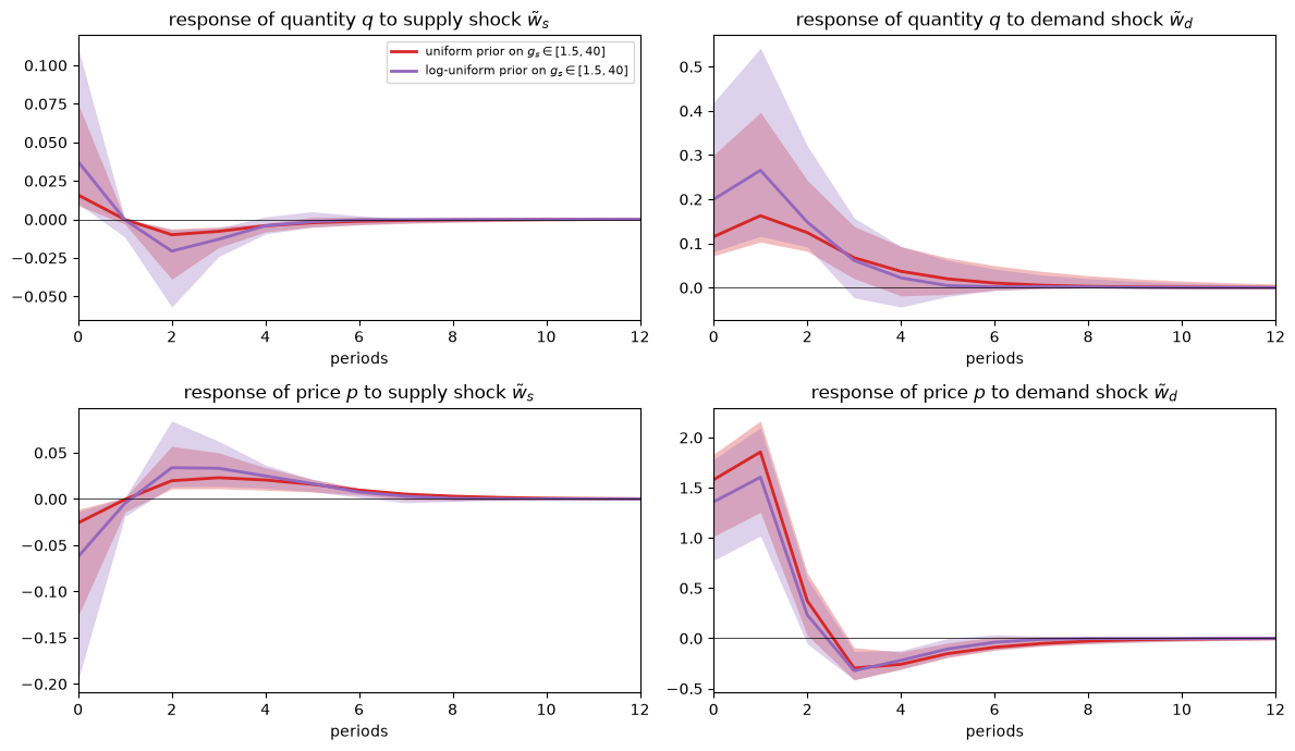
Fig. 28.15 Uniform versus log-uniform prior on \(g_s\)#
Moving prior mass toward small adjustment costs raises the median quantity responses to both shocks and widens their bands upward: economies in which suppliers adjust quickly now carry real prior weight.
What about the sign restrictions?
A sign holds with prior probability one if and only if it holds at every point of the support, apart from a set of prior probability zero.
Because both priors have positive density everywhere on the same support, they imply the same sign restrictions.
table_log = theory_signs(D_log)
print("same sign table under the uniform and log-uniform priors:",
      np.array_equal(table_log, table_w))
same sign table under the uniform and log-uniform priors: True
So the econometrician who imposes the theory’s sign restrictions does exactly the same thing under the two priors, and the map from \((g_s, g_d)\) to the three outcomes is the same.
What changes is how much prior probability falls in each region.
V_log, C_log = wide['log-uniform']['V'], wide['log-uniform']['C']
outcome_log = classify(C_log, V_log, D_log, table_log)

fig, ax = plt.subplots()
outcome_map(ax, gs_log, gd_log, outcome_log)
ax.set_xscale('log')
ax.set_xticks(gs_ticks, labels=[str(t) for t in gs_ticks])
ax.set_xlabel("$g_s$ (log scale)")
plt.tight_layout()
plt.show()

norms_log = np.linalg.norm(
    np.linalg.solve(np.linalg.cholesky(V_log), D_log[:, 0]), axis=1)
print(f"{'':12s} {'P(fundamental)':>15s}" +
      ''.join(f"{lab:>25s}" for lab in outcome_labels))
for name, nrm, out in [('uniform', norms_w, outcome),
                       ('log-uniform', norms_log, outcome_log)]:
    print(f"{name:12s} {np.mean(nrm[:, 0] > 0.99):15.2f}" +
          ''.join(f"{np.mean(out == c):25.2f}" for c in range(3)))
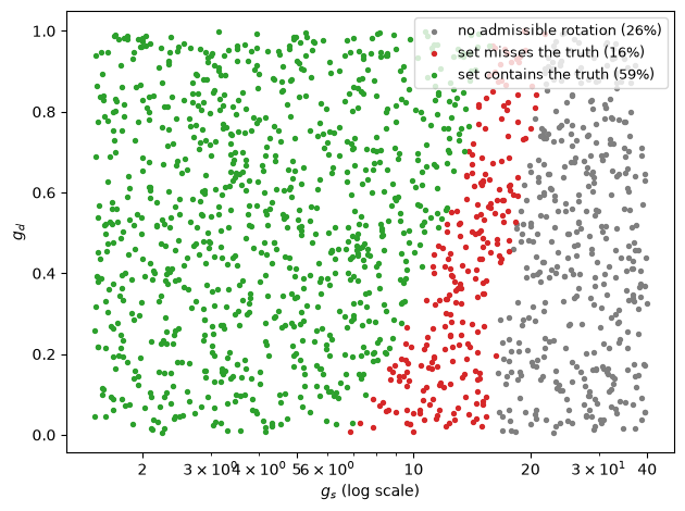
Fig. 28.16 Sign-restriction outcomes, log-uniform prior#
              P(fundamental)   no admissible rotation     set misses the truth   set contains the truth
uniform                 0.07                     0.58                     0.16                     0.25
log-uniform             0.30                     0.26                     0.16                     0.59
Here P(fundamental) is the prior probability \(\mathbb{P}\{\|L^{-1} d_s\| > 0.99\}\).
On a logarithmic axis the three regions are laid out evenly, and the green region — where the theory-implied sign restrictions recover the true supply response — is now the largest.
The same sign restrictions, derived from the same theory with the same parameter support, succeed with prior probability of roughly one quarter under one prior and about 60 percent under the other.
This complements a point that Baumeister and Hamilton [2015] make about the Haar prior over rotations: a prior that looks innocuous on one parameterization can be quite informative about the objects we care about.
Here the choice is between two equally “flat-looking” priors on a structural parameter, and it governs how likely we think it is that a VAR can recover the supply shock at all.
28.11. Summary#
A Bayesian structural modeler who is uncertain about two adjustment-cost parameters has, implicitly, a prior over every object that the model implies.
Monte Carlo makes those induced priors visible.
In our market:
The induced prior over structural impulse responses is concentrated and pins down a rich pattern of signs, many of which persist beyond the impact period.
The induced prior over the population VAR says that the innovations to price and quantity are almost perfectly correlated, with a covariance matrix slightly larger than that of the agents’ own surprises.
Under either Cholesky ordering, the first orthogonalized shock looks like the demand shock, but no orthogonalized shock looks like the supply shock.
Using the induced prior to generate sign restrictions in the spirit of Uhlig works well for the demand shock, which is essentially fundamental for \((q_t, p_t)\), and fails for the supply shock, which is not: imposing more correct restrictions shrinks the identified set onto the wrong answer.
Widening the prior produces bigger, and shifted, induced priors and weakens the restrictions the theory can license. Across the widest prior, sign restrictions recover the supply response only where suppliers adjust relatively quickly, so that the supply shock is fundamental or close to it; elsewhere the identified set misses the truth or is empty.
Changing the shape of the prior from uniform to log-uniform on the same support leaves the theory-implied sign restrictions unchanged — they depend only on the support — but moves prior mass toward fast-adjusting suppliers, and so raises the prior probability that those restrictions recover the supply response from roughly one quarter to about 60 percent.
The structural modeler, who believes the whole model, can do better.
With an infinite sample, the modeler can learn \((g_s, g_d)\) from the autocovariance function (see Exercise 28.3) and then compute the structural responses directly from the model, without ever rotating VAR innovations: if you know it, impose it.
28.12. Exercises#
Exercise 28.1
Exercise 2 of Dynamic Supply and Demand Curves showed that the market is (nearly) invertible when \(g_s \le 1\): quantity then adjusts quickly and reveals supply surprises at once.
Replace the prior on \(g_s\) by \(g_s \sim U[0.2, 1]\), keeping \(g_d \sim U[0.05, 0.15]\).
Recompute the induced prior over \(\|L^{-1} d_s\|\).
Recompute the sign table implied by the new prior.
Take \((g_s, g_d) = (0.6, 0.1)\) as the truth and apply Uhlig’s algorithm with the new table and \(K = 5\). Does the identified set now contain the true supply response?
Solution
We repeat the Monte Carlo with the new prior.
rng_ex = np.random.default_rng(42)
N_ex = 1_000
gs_ex = rng_ex.uniform(0.2, 1.0, N_ex)
gd_ex = rng_ex.uniform(g_d_lo, g_d_hi, N_ex)
draws_ex = [model_objects(gs, gd) for gs, gd in zip(gs_ex, gd_ex)]
D_ex = np.array([d['D'] for d in draws_ex])
V_ex = np.array([d['V'] for d in draws_ex])

norms_ex = np.linalg.norm(
    np.linalg.solve(np.linalg.cholesky(V_ex), D_ex[:, 0]), axis=1)
print(f"||L^-1 d_s|| in [{norms_ex[:, 0].min():.4f}, {norms_ex[:, 0].max():.4f}]")

pos_ex = (D_ex[:, :K_max + 1] > 0).mean(axis=0)
neg_ex = (D_ex[:, :K_max + 1] < 0).mean(axis=0)
table_ex = np.where(pos_ex == 1, 1, np.where(neg_ex == 1, -1, 0))
print("\nhorizon |  supply: q   p  |  demand: q   p")
for j in range(K_max + 1):
    s = [symbol[table_ex[j, i, k]] for k in range(2) for i in range(2)]
    print(f"   {j}    |     {s[0]}  {s[1]}   |     {s[2]}  {s[3]}")
||L^-1 d_s|| in [1.0000, 1.0000]

horizon |  supply: q   p  |  demand: q   p
   0    |      +    -    |      +    +
   1    |      -    +    |      +    +
   2    |      -    +    |      +    +
   3    |      -    +    |      ?    -
   4    |      ?    +    |      ?    -
   5    |      ?    +    |      -    -
The supply impact vector is now an admissible impulse vector, \(\|L^{-1} d_s\| \approx 1\).
Now we apply the sign restrictions at \((g_s, g_d) = (0.6, 0.1)\).
truth_ex = model_objects(0.6, 0.1)
kept_ex, acc_ex = sign_identified(truth_ex['C'], truth_ex['V'], table_ex, K_max)
print(f"acceptance rate: {acc_ex:.4f}")

lo, hi = kept_ex.min(0), kept_ex.max(0)
inside_ex = (lo - 1e-10 <= truth_ex['D']) & (truth_ex['D'] <= hi + 1e-10)
print("true supply response inside the set, horizons 0-7:")
print("  quantity:", inside_ex[:8, 0, 0])
print("  price:   ", inside_ex[:8, 1, 0])

fig, axes = plt.subplots(1, 2, figsize=(12, 4))
for i, ax in enumerate(axes):
    ax.fill_between(range(T), lo[:, i, 0], hi[:, i, 0], color='C3', alpha=0.3,
                    label=f'sign-identified set, K = {K_max}')
    ax.plot(truth_ex['D'][:, i, 0], 'k--', lw=2, label='true structural response')
    ax.axhline(0, color='k', lw=0.5)
    ax.set_title(f"response of {var_names[i]} to the supply shock, $g_s = 0.6$")
    ax.set_xlim(0, 12)
axes[0].legend()
plt.tight_layout()
plt.show()
acceptance rate: 0.0138
true supply response inside the set, horizons 0-7:
  quantity: [ True  True  True  True  True  True  True  True]
  price:    [ True  True  True  True  True  True  True  True]
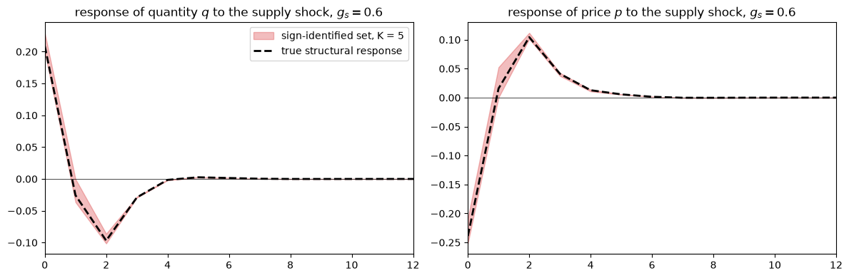
When the structural shocks are fundamental for \((q_t, p_t)\), the true structural responses are among the rotations of the VAR innovations, so correct sign restrictions produce an identified set that contains them.
Exercise 28.2
Uhlig’s Principle 6 [Uhlig, 2017] says that sign-restricting both shocks rather than one “can help: sometimes a lot, sometimes not at all”.
At the true parameters \((g_s, g_d) = (10, 0.1)\) and with \(K = 0\), compare the identified sets for the impact responses when you impose
only the restrictions on the supply shock,
only the restrictions on the demand shock,
both.
Which restriction does the work, and why?
Solution
We zero out the rows of the sign table that we don’t want to impose.
cases = {"supply only": [0], "demand only": [1], "both": [0, 1]}
for name, shocks in cases.items():
    tab = np.zeros_like(sign_table)
    tab[:, :, shocks] = sign_table[:, :, shocks]
    kept, acc = sign_identified(truth['C'], truth['V'], tab, 0)
    bounds = ([kept[:, 0, i, k].min() for k in range(2) for i in range(2)],
              [kept[:, 0, i, k].max() for k in range(2) for i in range(2)])
    print(f"{name:12s} acceptance {acc:.3f}")
    for (i, k), lo_, hi_ in zip([(0, 0), (1, 0), (0, 1), (1, 1)], *bounds):
        print(f"   impact of {shock_names[k][:6]} on {var_short[i]}: "
              f"[{lo_:7.4f}, {hi_:7.4f}]   truth {truth['D'][0, i, k]:7.4f}")
supply only  acceptance 0.062
   impact of supply on q: [ 0.0000,  0.0452]   truth  0.0326
   impact of supply on p: [-0.3193, -0.0007]   truth -0.0368
   impact of demand on q: [ 0.2283,  0.2328]   truth  0.2295
   impact of demand on p: [ 1.6121,  1.6434]   truth  1.6428
demand only  acceptance 0.940
   impact of supply on q: [ 0.0000,  0.2328]   truth  0.0326
   impact of supply on p: [-0.3193,  1.6434]   truth -0.0368
   impact of demand on q: [ 0.0000,  0.2328]   truth  0.2295
   impact of demand on p: [ 0.0004,  1.6434]   truth  1.6428
both         acceptance 0.062
   impact of supply on q: [ 0.0000,  0.0452]   truth  0.0326
   impact of supply on p: [-0.3193, -0.0007]   truth -0.0368
   impact of demand on q: [ 0.2283,  0.2328]   truth  0.2295
   impact of demand on p: [ 1.6121,  1.6434]   truth  1.6428
The supply restriction does almost all of the work.
Because the innovations are almost perfectly positively correlated, the data cloud lies close to a line with positive slope.
Only rotations that put the “supply” impulse vector nearly orthogonal to that line can make price and quantity move in opposite directions, and that forces the other impulse vector to lie almost along the line, which pins down the demand shock.
The demand restriction alone has little bite: almost every direction in the positive quadrant is consistent with it.
This is the case \(\mathrm{corr}(P, Q) \to 1\) in Figure 7 of Uhlig [2017].
Exercise 28.3
The structural modeler believes the whole model.
Suppose the modeler sees an infinite sample from the economy at \((g_s, g_d) = (10, 0.1)\), and therefore knows the autocovariances \(\Gamma_0, \ldots, \Gamma_{T-1}\).
On a grid of values \((g_s, g_d)\) covering the support of the prior, compute the distance
and show that it has a unique minimum at the true values.
What does this imply about the modeler’s posterior in an infinite sample, and about the posterior over the structural impulse responses?
Solution
gs_grid = np.linspace(g_s_lo, g_s_hi, 21)
gd_grid = np.linspace(g_d_lo, g_d_hi, 21)
Γ_target = truth['Γ']

dist = np.empty((len(gs_grid), len(gd_grid)))
for m, gs in enumerate(gs_grid):
    for n, gd in enumerate(gd_grid):
        dist[m, n] = np.sum((model_objects(gs, gd)['Γ'] - Γ_target)**2)

m, n = np.unravel_index(dist.argmin(), dist.shape)
print(f"minimizer on the grid: g_s = {gs_grid[m]:.2f}, g_d = {gd_grid[n]:.3f}")

fig, ax = plt.subplots(figsize=(7, 5))
cs = ax.contourf(gd_grid, gs_grid, np.log10(np.maximum(dist, 1e-6)), levels=30)
ax.plot(g_d_true, g_s_true, 'w*', ms=14)
ax.set_xlabel("$g_d$")
ax.set_ylabel("$g_s$")
ax.set_title("$\\log_{10}$ distance between autocovariance functions")
fig.colorbar(cs)
plt.tight_layout()
plt.show()
minimizer on the grid: g_s = 10.00, g_d = 0.100
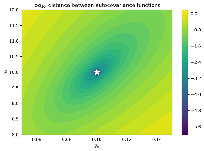
The autocovariance function identifies \((g_s, g_d)\).
The elongated valley shows that the autocovariances are less sensitive to movements in which \(g_s\) and \(g_d\) rise together than to movements in which they go in opposite directions, so a finite sample would leave the modeler with a positively correlated posterior.
In an infinite sample the modeler’s likelihood concentrates on the true values, so the posterior over \((g_s, g_d)\) collapses to a point mass at \((10, 0.1)\), and so does the posterior over the structural impulse responses, since they are a function of \((g_s, g_d)\).
The modeler learns the true supply response exactly, including the part that no rotation of VAR innovations can deliver, because the modeler does not use VAR rotations: the model maps the parameters directly into the responses.
This is the payoff from Uhlig’s first principle, if you know it, impose it.
The sign-restriction econometrician, who imposes less, learns less, and in this market learns something wrong about the supply shock.
Exercise 28.4
The widest prior on \(g_d\), \(U[0.005, 1]\), spans an even wider range, a factor of 200.
Put log-uniform priors on both \(g_s \in [1.5, 40]\) and \(g_d \in [0.005, 1]\).
Check that the theory-implied sign table is unchanged.
Compute the prior probabilities of the three sign-restriction outcomes and compare them with those under the uniform prior and under the prior that is log-uniform in \(g_s\) only.
Explain the direction of the change, using the outcome maps above.
Solution
rng_ll = np.random.default_rng(99)
gs_ll = np.exp(rng_ll.uniform(np.log(1.5), np.log(40.0), N_wide))
gd_ll = np.exp(rng_ll.uniform(np.log(0.005), np.log(1.0), N_wide))
objs = [model_objects(x, y) for x, y in zip(gs_ll, gd_ll)]
D_ll = np.array([o['D'] for o in objs])
V_ll = np.array([o['V'] for o in objs])
C_ll = np.array([o['C'] for o in objs])

print("same sign table:", np.array_equal(theory_signs(D_ll), table_w))
outcome_ll = classify(C_ll, V_ll, D_ll, table_w)

print(f"\n{'':22s}" + ''.join(f"{lab:>25s}" for lab in outcome_labels))
for name, out in [('uniform, uniform', outcome),
                  ('log-uniform, uniform', outcome_log),
                  ('log-uniform, log-unif.', outcome_ll)]:
    print(f"{name:22s}" + ''.join(f"{np.mean(out == c):25.2f}" for c in range(3)))

fig, ax = plt.subplots(figsize=(9, 5))
outcome_map(ax, gs_ll, gd_ll, outcome_ll,
            "log-uniform priors on $g_s$ and $g_d$: sign restrictions, K = 5")
ax.set_xscale('log')
ax.set_yscale('log')
ax.set_xticks(gs_ticks, labels=[str(t) for t in gs_ticks])
ax.set_xlabel("$g_s$ (log scale)")
ax.set_ylabel("$g_d$ (log scale)")
plt.tight_layout()
plt.show()
same sign table: True

                         no admissible rotation     set misses the truth   set contains the truth
uniform, uniform                           0.58                     0.16                     0.25
log-uniform, uniform                       0.26                     0.16                     0.59
log-uniform, log-unif.                     0.29                     0.21                     0.51
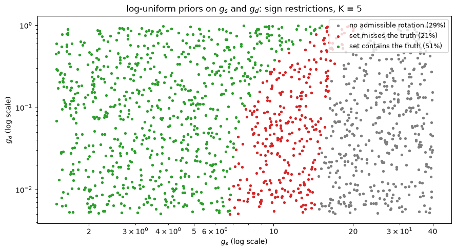
The sign table is unchanged because the support is unchanged.
A log-uniform prior on \(g_d\) shifts mass toward small values of \(g_d\).
The outcome maps show that the green region extends to larger values of \(g_s\) when \(g_d\) is large: the boundary between the green and red regions slopes upward.
Moving prior mass toward small \(g_d\) therefore moves mass out of the green region, and the probability that the sign restrictions recover the supply response falls relative to the prior that is log-uniform in \(g_s\) alone, though it stays well above its value under the uniform prior.