
29. Policy Counterfactuals from Impulse Responses#
29.1. Overview#
How would an economy respond to its shocks if policy followed a different rule from the one that generated the historical data used to estimate a model?
Lucas [1976] taught us that a reliable answer requires a model whose private-sector decision rules change appropriately when the policy rule changes.
McKay and Wolf [2023] claim that, in a particular class of linear models, an econometrician can construct such Lucas-critique-robust counterfactuals without writing down the model.
The econometrician needs instead what they call “dynamic causal effects” of policy shocks — surprise deviations from a prevailing policy rule, both contemporaneous and anticipated (“news”) — together with the effects of the non-policy shock of interest under the prevailing policy rule.
This lecture puts their result to work in the context of a generalized version of the market for a single good studied in Dynamic Supply and Demand Curves and Induced Priors for Impulse Responses.
The market in those lectures has no policy of the type that concerns McKay and Wolf; we add one here: a per-unit tax on the good that the government adjusts according to a rule that leans against movements in the price.
The lecture
shows that the market with a tax fits McKay and Wolf’s framework, and that their key assumption is precisely the invariance of the open-loop dynamic supply and demand curves of Dynamic Supply and Demand Curves,
verifies their identification result: impulse responses to tax shocks under one rule deliver the economy’s exact behavior under another rule,
compares it with the older approach of Sims and Zha [2006], which imposes the new rule with a sequence of policy surprises and so falls foul of the Lucas critique, and examines a version of the defense of that approach by Leeper and Zha [2003] for “modest” policy interventions,
compares McKay and Wolf’s sufficient statistics with the counterfactuals of a structural modeler, who must commit to a parametric model of the private sector, as in Induced Priors for Impulse Responses,
asks what the econometrician can do with less than the full set of sufficient statistics: evidence on only a few policy shocks, data generated under a different rule, and, as Caravello et al. [2026] propose, a model fitted to the evidence to fill in the rest,
computes optimal policy under commitment and under discretion from the same objects, and
relates McKay and Wolf’s approach to the “dynamic programming squared” response to the Lucas critique and states what their counterfactuals take for granted.
Invertibility and Policy Counterfactuals asks what it takes to estimate the impulse responses that McKay and Wolf’s method uses, a question that connects this lecture to Dynamic Supply and Demand Curves and Induced Priors for Impulse Responses, in which the supply shock is not fundamental for prices and quantities.
29.2. A market with a tax#
We use the market of Dynamic Supply and Demand Curves with the same parameter values.
Its supply side — competitive firms facing quadratic costs of adjusting output, with each firm taking the market price as given — is a close cousin of the model in Rational Expectations Equilibrium, where the “big \(Y\), little \(y\)” device corresponds to the “big \(X\), little \(x\)” device of Dynamic Supply and Demand Curves.
h_s = h_d = 1.0
g_s, g_d = 10.0, 0.1
β = 1 / 1.05
a = np.array([1, .8, .6, .4, .2])       # a(L): coefficients a0..a4

# MA polynomials for the shocks (coefficients on L^0..L^3)
B_d = np.convolve(np.convolve([1, .6], [1, .4]), [1, .2])
B_s = np.convolve(np.convolve([1, -.8], [1, .4]), [1, .2])

σ_s, σ_d = np.sqrt(0.5), 2.0            # shock standard deviations
As in Induced Priors for Impulse Responses, we work with a favorable supply shock \(\tilde w_{st} = -w_{st}\) and a positive demand shock \(\tilde w_{dt} = -w_{dt}\), each one standard deviation in size, so that both raise quantity.
The government levies a tax \(\tau_t\) per unit of the good, paid by suppliers, so that suppliers receive \(p_t - \tau_t\) when demanders pay \(p_t\); a negative \(\tau_t\) is a subsidy.
The supplier now maximizes
while the demander’s problem is unchanged.
The two Euler equations become
and eliminating \(p_t\) gives the market Euler equation \(\mathbb{E}_t\, \psi(L) q_t = -(s_t + d_t + \tau_t)\), with \(\psi(L) = h_s + h_d + g_s(1-\beta L^{-1})(1-L) + g_d\, a(\beta L^{-1})a(L)\), in which the tax enters exactly like a shock.
The government sets the tax by the rule
With \(\phi > 0\) the government subsidizes the good when its price is high and taxes it when its price is low, which stabilizes the price.
The policy shock \(\nu_{\ell, t-\ell}\) is a deviation from the rule at date \(t\) that was announced at date \(t - \ell\): \(\nu_{0,t}\) is a contemporaneous surprise, while \(\nu_{\ell, t-\ell}\) with \(\ell > 0\) is news about future policy.
29.2.1. The McKay–Wolf framework#
McKay and Wolf write a linear economy as two blocks,
where a variable written without a time subscript denotes its entire time path, as in \(x = (x_0, x_1, \ldots)\).
Here \(x\) collects observable outcomes, \(z\) the policy instrument, \(\varepsilon\) the non-policy shocks, and \(\nu\) the full menu of contemporaneous and news policy shocks; these are McKay and Wolf’s symbols, and we change them slightly below.
Their key assumption is that the private-sector block — the matrices \(H\) — does not depend on the coefficients \((A_x, A_z)\) of the policy rule: policy affects private decisions only through the expected path of the instrument.
Our market satisfies this assumption, with observables \((q, p)\), instrument \(z = \tau\), and no unobserved endogenous variables \(w\).
To keep notation light, from now on we stack the observables and the instrument into one vector of paths, \(x = (q, p, \tau)\), path by path: first \(q_0, \ldots, q_{T-1}\), then the prices, then the taxes.
We write the policy rule as \(R\, x = \nu\).
The private-sector block consists of the Euler equations (29.1)–(29.2), which do not involve \(\phi\).
These are the open-loop dynamic supply and demand curves of Dynamic Supply and Demand Curves, valid for an arbitrary path of prices — and now taxes — that the agents take as given.
The closed-loop decision rules that obtain inside a rational expectations equilibrium do depend on \(\phi\), because the equilibrium price process does: that dependence is the Lucas critique.
McKay and Wolf’s assumption would fail if, for example, agents had less information than the government and had to infer something about the economy from the tax rate.
Then the coefficients of the policy rule would affect what agents learn from observing the tax, as in the environments of Knowing the Forecasts of Others, where decision makers extract signals about hidden states from equilibrium prices and quantities.
In our market, agents see the shocks \(w_{st}, w_{dt}\) and know the policy rule.
29.2.2. Solving in sequence space#
Because the economy is linear, the impulse response to a shock that occurs at date 0 is the perfect-foresight path that follows it, with the shock’s entire future consequences — including any announced future deviations from the rule — known at date 0.
Following McKay and Wolf, we compute such paths by stacking the equations for \(t = 0, 1, \ldots, T-1\) into one linear system.
We set \(q_t = 0\) for \(t < 0\) (the economy starts at its steady state) and for \(t \ge T\) (impulse responses have died out by date \(T\)).
This is the finite-horizon approach of Classical Control with Linear Algebra: the stacked first-order conditions form one banded linear system, and as \(T\) grows its solution converges to the infinite-horizon solution that Dynamic Supply and Demand Curves obtains by factoring the characteristic polynomial into stable and unstable parts.
The terminal condition \(q_t = 0\) for \(t \ge T\) selects the bounded solution.
McKay and Wolf assume that both the baseline and the counterfactual rules deliver a unique bounded equilibrium.
Caravello et al. [2026] drop that assumption for the counterfactual rule, as Policy Counterfactuals in a New Keynesian Economy explains; every rule that we study in this market delivers a unique bounded equilibrium, for a reason given in Price stabilization as more flexible supply, and we check below that our answers do not depend on \(T\).
The term \(g_d a(\beta L^{-1}) a(L) q_t\) in (29.2) equals \(g_d \sum_{i=0}^4 \sum_{k=0}^4 a_i a_k \beta^i q_{t+i-k}\).
T = 200     # length of the stacked paths

def private_block(g_s, g_d, T=T, h_s=h_s):
    """
    Stack the Euler equations for t = 0, ..., T-1.

    Unknowns are ordered x = (q, p, τ), each a path of length T, and the
    equations read  H @ x = (s, -d).
    """
    Φ_s, Φ_d = np.zeros((T, T)), np.zeros((T, T))
    for t in range(T):
        Φ_s[t, t] += h_s + g_s * (1 + β)
        if t >= 1:
            Φ_s[t, t - 1] -= g_s
        if t + 1 < T:
            Φ_s[t, t + 1] -= g_s * β
        Φ_d[t, t] += h_d
        for i in range(5):
            for k in range(5):
                if 0 <= t + i - k < T:
                    Φ_d[t, t + i - k] += g_d * a[i] * a[k] * β**i
    I, O = np.eye(T), np.zeros((T, T))
    return np.block([[-Φ_s, I, -I],      # supply:  p - τ - Φ_s q = s
                     [Φ_d, I, O]])       # demand:  p + Φ_d q = -d

def rule_block(φ, T=T):
    "The rule τ = -φ p + ν written as  R @ x = ν."
    return np.hstack([np.zeros((T, T)), φ * np.eye(T), np.eye(T)])

def system_inverse(g_s, g_d, φ, h_s=h_s):
    "Inverse of the stacked system: x = inverse @ (s, -d, ν)."
    return np.linalg.inv(np.vstack([private_block(g_s, g_d, h_s=h_s), rule_block(φ)]))

def forcing(shock, T=T, σ_s=σ_s):
    "Right-hand side for a favorable supply shock (0) or a positive demand shock (1)."
    s, d = np.zeros(T), np.zeros(T)
    if shock == 0:
        s[:4] = -σ_s * B_s
    else:
        d[:4] = -σ_d * B_d
    return np.concatenate([s, -d, np.zeros(T)])

def split(x):
    "Split a stacked path into (q, p, τ)."
    return x[:T], x[T:2 * T], x[2 * T:]
To check that the truncation does not matter, we solve for the response to a demand shock with \(T = 150\) and \(T = 300\) under three very different rules and compare the first 40 periods of quantity, price, and the tax.
for φ in [-0.5, 0.5, 10.0]:
    paths = []
    for T_check in [150, 300]:
        M_check = np.vstack([private_block(g_s, g_d, T_check), rule_block(φ, T_check)])
        x_check = np.linalg.solve(M_check, forcing(1, T_check))
        paths.append(np.concatenate([x_check[b * T_check:b * T_check + 40] for b in range(3)]))
    print(f"φ = {φ:5}: max |T=150 - T=300| = {np.abs(paths[0] - paths[1]).max():.1e}")
φ =  -0.5: max |T=150 - T=300| = 4.4e-16
φ =   0.5: max |T=150 - T=300| = 8.9e-16
φ =  10.0: max |T=150 - T=300| = 4.4e-15
Before going on, we check that with no tax (\(\phi = 0\), \(\nu = 0\)) the sequence-space solution reproduces the optimal-linear-regulator solution of Dynamic Supply and Demand Curves, whose code we repeat in the hidden cell below.
shock 0: max |sequence space - regulator| over 30 periods = 2.2e-06
shock 1: max |sequence space - regulator| over 30 periods = 1.7e-05
The two methods agree up to the tiny ridge that regularizes the regulator’s Riccati equation.
29.3. How the policy rule shapes the response to shocks#
We take \(\phi = 0.5\) as the baseline rule that has prevailed historically, and compare it with no policy (\(\phi = 0\)) and with aggressive price stabilization (\(\phi = 2\)).
φ_A = 0.5                      # baseline rule
H_plot = 20                    # horizons to plot
names = ["quantity $q$", "price $p$", "tax $\\tau$"]
shock_names = ["supply shock $\\tilde w_s$", "demand shock $\\tilde w_d$"]

fig, axes = plt.subplots(3, 2, figsize=(12, 9))
for φ, ls in [(0.0, ':'), (φ_A, '-'), (2.0, '--')]:
    M_inv = system_inverse(g_s, g_d, φ)
    for k in range(2):
        paths = split(M_inv @ forcing(k))
        for i in range(3):
            axes[i, k].plot(paths[i][:H_plot], ls, lw=2, label=f"$\\phi = {φ}$")
for i in range(3):
    for k in range(2):
        axes[i, k].axhline(0, color='k', lw=0.5)
        axes[i, k].set_title(f"response of {names[i]} to {shock_names[k]}")
axes[0, 0].legend()
for ax in axes[-1]:
    ax.set_xlabel("periods")
plt.tight_layout()
plt.show()
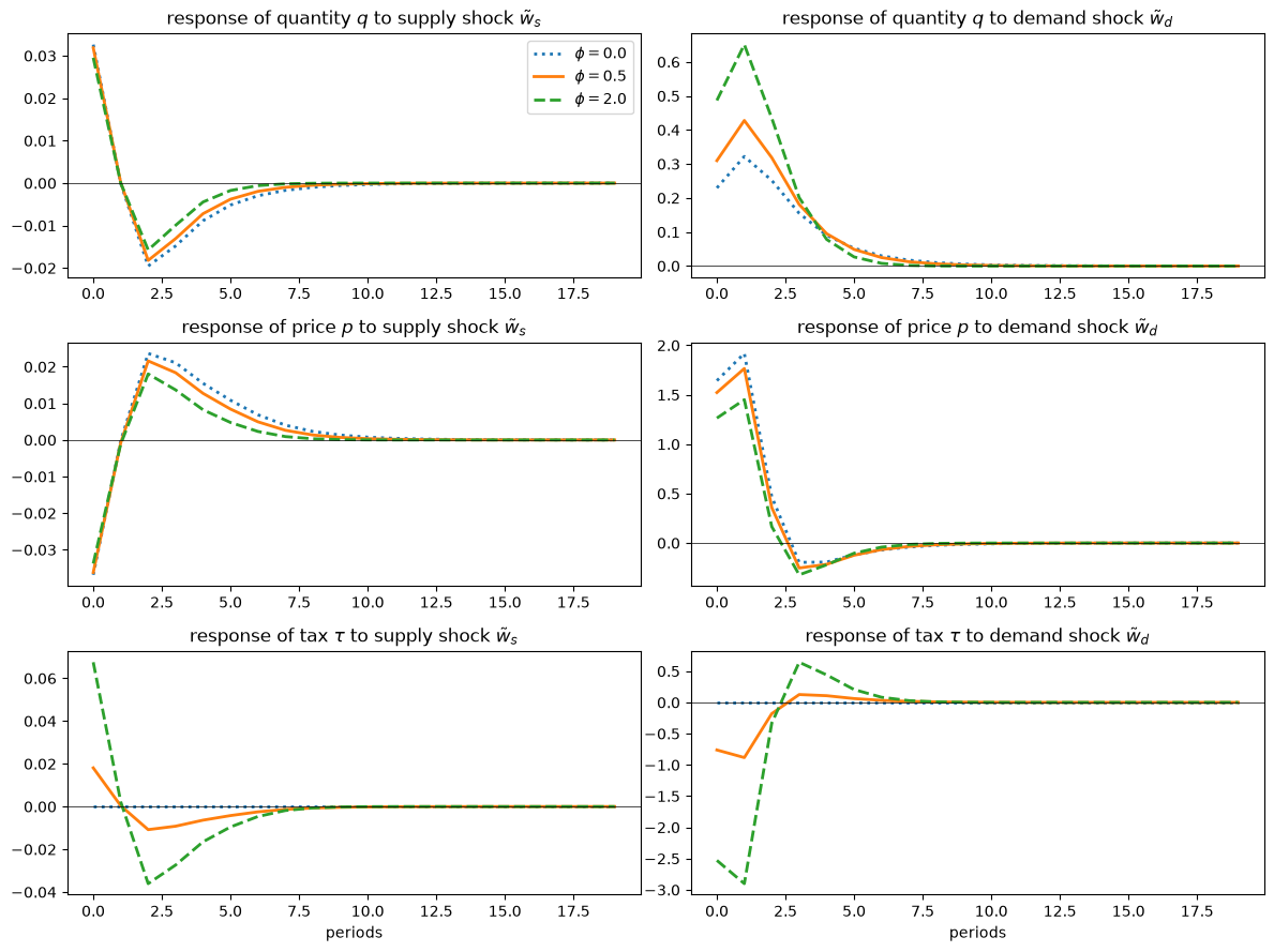
Fig. 29.1 Responses under three policy rules#
A more aggressive rule damps the price response to a demand shock by subsidizing the good when its price rises, and quantity rises by more.
Every one of these responses reflects how forward-looking suppliers and demanders adjust their plans to the rule: the closed-loop decision rules change with \(\phi\).
29.3.1. Price stabilization as more flexible supply#
When \(\tau_t = -\phi p_t\), suppliers receive \(p_t - \tau_t = (1 + \phi) p_t\), and the supply Euler equation (29.1) becomes
Dividing by \(1 + \phi\) shows that, as far as \((q_t, p_t)\) are concerned, the market with the tax rule behaves exactly like a market without a tax whose supplier has
To someone who observes only prices and quantities, a price-stabilizing rule is indistinguishable from suppliers who are more flexible — with lower costs of producing and of adjusting output — and who face smaller cost shocks.
(Someone who also observes the tax can tell the two markets apart.)
The same algebra applies to any rule with \(\phi > -1\); for \(-1 < \phi < 0\), a rule that destabilizes the price, the equivalent suppliers are less flexible.
The equivalence also explains why every such rule delivers a unique equilibrium: the equilibrium of the untaxed market solves a planning problem with a strictly convex objective (Dynamic Supply and Demand Curves).
We confirm the equivalence numerically.
for φ in [0.5, 2.0]:
    gaps = []
    for shock in range(2):
        q1, p1, _ = split(system_inverse(g_s, g_d, φ) @ forcing(shock))
        q2, p2, _ = split(system_inverse(g_s / (1 + φ), g_d, 0.0, h_s=h_s / (1 + φ))
                          @ forcing(shock, σ_s=σ_s / (1 + φ)))
        gaps.append(max(np.abs(q1 - q2).max(), np.abs(p1 - p2).max()))
    print(f"φ = {φ}: max |rule economy - flexible-supply economy| = {max(gaps):.1e}")
φ = 0.5: max |rule economy - flexible-supply economy| = 2.0e-15
φ = 2.0: max |rule economy - flexible-supply economy| = 1.8e-15
The equivalence explains a feature of the previous figure: under a more aggressive rule, quantity responds more strongly to a demand shock, just as it would if suppliers could adjust output more easily.
The equivalence also states the Lucas critique compactly in our market.
An econometrician who fit the dynamic supply curve to data generated under the rule, ignoring the tax, would estimate the cost parameters \(h_s/(1+\phi)\) and \(g_s/(1+\phi)\), not \(h_s\) and \(g_s\), and would mispredict what happens if the rule changes.
29.4. McKay and Wolf’s identification result#
Their result combines two ingredients measured under the baseline rule: the responses to policy shocks, which we compute first, and the response to the non-policy shock of interest.
29.4.1. The causal effects of policy shocks#
A policy shock \(\nu_{\ell,0}\) announces at date 0 that the tax will deviate from the rule at date \(\ell\).
Column \(\ell\) of the matrix \(\Theta_{\nu}\) below collects the responses of \((q, p, \tau)\) to such a shock of size one under the baseline rule.
M_inv_A = system_inverse(g_s, g_d, φ_A)
Θ_ν = M_inv_A[:, 2 * T:]          # 3T x T: responses to news at every horizon

fig, axes = plt.subplots(1, 3, figsize=(14, 4))
for ℓ, color in zip([0, 4, 8], ['C0', 'C1', 'C2']):
    paths = split(Θ_ν[:, ℓ])
    label = "surprise ($\\ell = 0$)" if ℓ == 0 else f"news about date {ℓ}"
    for i in range(3):
        axes[i].plot(paths[i][:H_plot], color=color, lw=2, label=label)
for i in range(3):
    axes[i].axhline(0, color='k', lw=0.5)
    axes[i].set_title(f"response of {names[i]}")
    axes[i].set_xlabel("periods")
axes[0].legend()
plt.tight_layout()
plt.show()
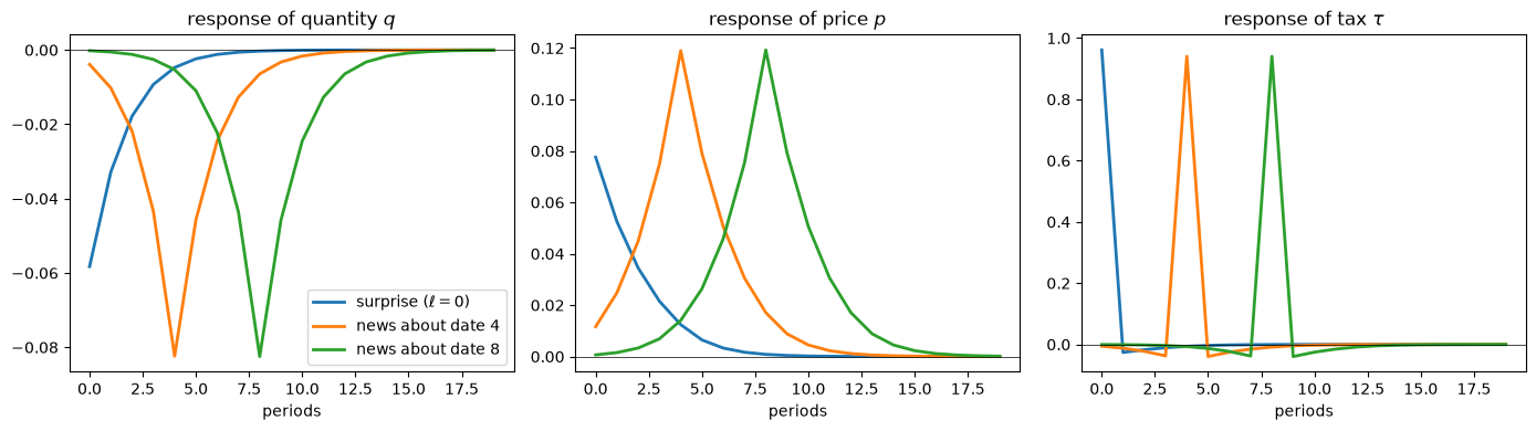
Fig. 29.2 Responses to tax surprises and news#
News of a future tax increase lowers quantity well before the tax rises: suppliers, who find it costly to adjust output, begin cutting it as soon as they learn of the tax.
These anticipation effects make the whole policy path matter for private decisions.
29.4.2. Proposition 1#
Let \(x_A(\varepsilon)\) be the response of \(x = (q, p, \tau)\) to a non-policy shock \(\varepsilon\) under the baseline rule, and consider a counterfactual rule \(\tau_t = -\tilde\phi\, p_t\), written as \(\tilde R\, x = 0\).
McKay and Wolf’s Proposition 1 says that the counterfactual response is given by the formula below, where, following their notation, the subscript \(A\) marks the baseline rule and \(\tilde A\) the counterfactual rule \(\tilde R\):
The logic is that suppliers and demanders care only about the expected path of the tax.
A date-0 combination of contemporaneous and news shocks \(\tilde\nu\) can produce any expected tax path, in particular the one that the counterfactual rule would produce.
Because the shocks are all announced at date 0, the new rule holds both ex post along the path and ex ante, in agents’ expectations from date 0 on.
The econometrician needs \(x_A(\varepsilon)\) and \(\Theta_\nu\) — objects that can be estimated from data generated under the baseline rule — but not the model’s equations, nor even the baseline rule.
def mw_counterfactual(M_inv_base, x_A, φ_new):
    "McKay–Wolf Proposition 1: enforce τ = -φ_new p with date-0 policy shocks."
    Θ = M_inv_base[:, 2 * T:]
    R_new = rule_block(φ_new)
    ν = np.linalg.solve(R_new @ Θ, -R_new @ x_A)
    return x_A + Θ @ ν, ν
29.4.3. The Sims–Zha alternative#
Sims and Zha [2006] proposed to enforce a counterfactual rule with a single kind of policy shock, the contemporaneous surprise \(\nu_{0,t}\), choosing a new value at each date so that the rule holds period by period.
This uses less information — only the first column of \(\Theta_\nu\) — but the rule then holds only ex post: at each date, agents expect the baseline rule to apply in the future and are surprised again and again.
A surprise at date \(t\) has the same effects as one at date 0, shifted \(t\) periods, and no effect before date \(t\).
def sims_zha(M_inv_A, x_A, φ_new):
    "Enforce τ = -φ_new p ex post with a sequence of contemporaneous surprises."
    θ0 = M_inv_A[:, 2 * T]                # response to a date-0 surprise
    Θ_sz = np.zeros((3 * T, T))
    for t in range(T):
        for b in range(3):                # shift each block (q, p, τ) by t periods
            Θ_sz[b * T + t:(b + 1) * T, t] = θ0[b * T:(b + 1) * T - t]
    R_new = rule_block(φ_new)
    ν = np.linalg.solve(R_new @ Θ_sz, -R_new @ x_A)
    return x_A + Θ_sz @ ν, ν
We compute the response to a demand shock under aggressive price stabilization, \(\tilde\phi = 2\), in three ways: by solving the model under the new rule (the truth), by McKay and Wolf’s method, and by Sims and Zha’s.
φ_new = 2.0
x_A = M_inv_A @ forcing(1)
x_true = system_inverse(g_s, g_d, φ_new) @ forcing(1)
x_mw, ν_mw = mw_counterfactual(M_inv_A, x_A, φ_new)
x_sz, ν_sz = sims_zha(M_inv_A, x_A, φ_new)

print(f"max |McKay–Wolf - truth| = {np.abs(x_mw - x_true).max():.1e}")
print(f"max |Sims–Zha   - truth| = {np.abs(x_sz - x_true).max():.1e}")

fig, axes = plt.subplots(1, 4, figsize=(16, 4))
for i in range(3):
    ax = axes[i]
    ax.plot(split(x_A)[i][:H_plot], 'k:', lw=2, label=f"baseline rule $\\phi = {φ_A}$")
    ax.plot(split(x_true)[i][:H_plot], 'C0', lw=2, label=f"true, $\\tilde\\phi = {φ_new}$")
    ax.plot(split(x_mw)[i][:H_plot], 'C0o', ms=4, label="McKay–Wolf")
    ax.plot(split(x_sz)[i][:H_plot], 'C3--', lw=2, label="Sims–Zha")
    ax.axhline(0, color='k', lw=0.5)
    ax.set_title(f"{names[i]}, demand shock")
    ax.set_xlabel("periods")
axes[0].legend(fontsize=8)
axes[3].bar(np.arange(H_plot) - 0.2, ν_mw[:H_plot], width=0.4, color='C0',
            label="McKay–Wolf: news at date 0 about date $t$")
axes[3].bar(np.arange(H_plot) + 0.2, ν_sz[:H_plot], width=0.4, color='C3',
            label="Sims–Zha: surprise at date $t$")
axes[3].axhline(0, color='k', lw=0.5)
axes[3].set_title("policy shocks used")
axes[3].set_xlabel("$t$")
axes[3].legend(fontsize=8)
plt.tight_layout()
plt.show()
max |McKay–Wolf - truth| = 6.7e-16
max |Sims–Zha   - truth| = 2.0e-01
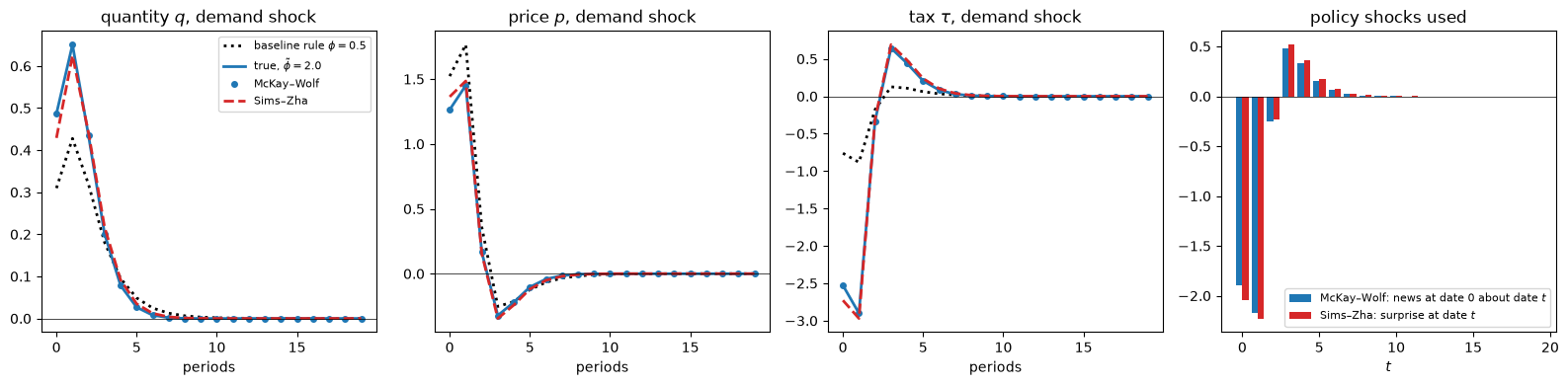
Fig. 29.3 Counterfactual responses to a demand shock#
McKay and Wolf’s construction reproduces the true counterfactual to machine precision.
The Sims–Zha construction does not: because suppliers and demanders keep expecting the old rule, they plan for less price stabilization than they actually get.
The fourth panel shows how close the two constructions are in the shocks they use.
McKay and Wolf’s shocks are \((-1.90, -2.18, -0.25, 0.48, \ldots)\) and Sims and Zha’s are \((-2.05, -2.23, -0.23, 0.52, \ldots)\): nearly the same numbers.
The difference is when agents learn them.
McKay and Wolf announce the whole sequence at date 0, as news about dates \(t = 0, 1, \ldots\); Sims and Zha spring each one as a surprise at date \(t\).
Here the Lucas critique operates through that difference in timing; even the small differences between the two sequences come from it.
Because the error comes from expectations, we expect it to grow with the weight that agents place on the future, and the supplier’s adjustment cost \(g_s\) governs how forward-looking supply is.
We compute, for a range of values of \(g_s\), the error in the counterfactual response to a demand shock when the rule moves from \(\phi_A = 0.5\) to \(\tilde\phi = 2\).
g_grid = np.geomspace(0.1, 30, 12)

def sz_error_curve(g_d_):
    "Largest relative Sims–Zha errors in (q, p) across the grid of supplier adjustment costs."
    out = []
    for g in g_grid:
        M_inv = system_inverse(g, g_d_, φ_A)
        x_A_g = M_inv @ forcing(1)
        x_true_g = system_inverse(g, g_d_, φ_new) @ forcing(1)
        x_sz_g, _ = sims_zha(M_inv, x_A_g, φ_new)
        out.append([np.abs(split(x_sz_g)[i] - split(x_true_g)[i]).max()
                    / np.abs(split(x_true_g)[i]).max() for i in range(2)])
    return np.array(out)

sz_errors = sz_error_curve(g_d)
sz_errors_static = sz_error_curve(0.0)

fig, ax = plt.subplots()
ax.semilogx(g_grid, sz_errors[:, 0], 'o-', lw=2, label="quantity")
ax.semilogx(g_grid, sz_errors[:, 1], 's-', lw=2, label="price")
ax.semilogx(g_grid, sz_errors_static[:, 0], 'C0--', lw=1.5, label="quantity, static demand ($g_d = 0$)")
ax.axvline(g_s, color='k', ls=':', lw=1)
ax.set_xlabel("supplier's adjustment cost $g_s$ (log scale)")
ax.set_ylabel("max relative error")
ax.legend()
plt.tight_layout()
plt.show()
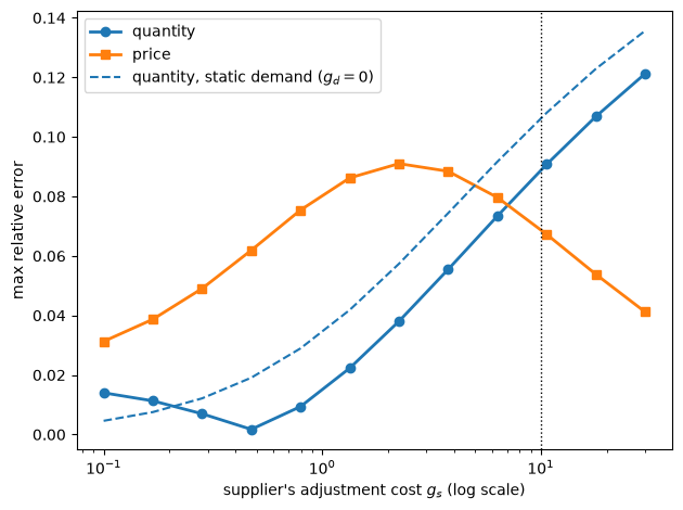
Fig. 29.4 Sims–Zha error and adjustment costs#
Beyond very small values of \(g_s\), the error in quantity rises with \(g_s\): the more slowly suppliers can adjust, the more their current decisions depend on expected future policy, and the more it matters that the Sims–Zha counterfactual gets those expectations wrong.
For \(g_s\) below about 0.5, the error in quantity falls as \(g_s\) rises.
The error combines two expectational errors of opposite sign, the demanders’ and the suppliers’.
With \(g_d = 0.1\), the demanders’ error dominates when \(g_s\) is very small, so that the Sims–Zha counterfactual overstates the response of quantity on impact; the suppliers’ error dominates when \(g_s\) is large, so that it understates it; and the two nearly cancel near \(g_s = 0.5\).
With static demand (\(g_d = 0\), the dashed line), only the suppliers’ error remains, and the error in quantity rises with \(g_s\) throughout.
The dotted vertical line marks our baseline value \(g_s = 10\).
The relative error in the price peaks near \(g_s = 2\) and then falls, although the absolute error keeps growing until \(g_s\) is about 7 and stays near 0.10 out to \(g_s = 10\): when adjustment costs are large, quantity is sluggish, the demand shock falls mostly on the price, and the price response grows faster than the error.
29.4.4. Modest policy interventions#
Leeper and Zha [2003] offered a defense of the Sims–Zha approach: if a policy intervention is modest, then ignoring its effect on expectations should do little harm.
Their notion of modesty is statistical: an intervention is modest if the policy shocks that implement it are small relative to the historical variability of policy shocks, so that agents would not detect a change in the policy regime.
Their statistic compares the implementing shocks with the historical variance of policy shocks, which our market does not specify.
Our market lets us examine a closely related question: how does the Sims–Zha error behave as the counterfactual rule \(\tilde\phi\) approaches the baseline \(\phi_A = 0.5\), so that the shocks needed to implement it shrink toward zero?
We compare the error with the size of the effect being estimated, the difference between the counterfactual and the baseline responses.
φ_tildes = np.array([0.4, 0.45, 0.48, 0.52, 0.55, 0.6, 0.75, 1.0, 2.0, 4.0])
ratios, sizes = [], []
for φ_t in φ_tildes:
    x_true_t = system_inverse(g_s, g_d, φ_t) @ forcing(1)
    x_sz_t, _ = sims_zha(M_inv_A, x_A, φ_t)
    effect = np.abs(split(x_true_t)[0] - split(x_A)[0]).max()
    error = np.abs(split(x_sz_t)[0] - split(x_true_t)[0]).max()
    sizes.append(effect)
    ratios.append(error / effect)

fig, axes = plt.subplots(1, 2, figsize=(12, 4))
axes[0].plot(φ_tildes, sizes, 'o-', lw=2, label="policy effect on $q$")
axes[0].plot(φ_tildes, np.array(ratios) * np.array(sizes), 's-', lw=2, label="Sims–Zha error in $q$")
axes[0].set_xlabel("counterfactual rule $\\tilde\\phi$")
axes[0].set_title("absolute size")
axes[0].legend()
axes[1].plot(φ_tildes, ratios, 'o-', lw=2, color='C3')
axes[1].set_ylim(0, 0.4)
axes[1].set_xlabel("counterfactual rule $\\tilde\\phi$")
axes[1].set_title("Sims–Zha error / policy effect")
for ax in axes:
    ax.axvline(φ_A, color='k', ls=':', lw=1)
plt.tight_layout()
plt.show()
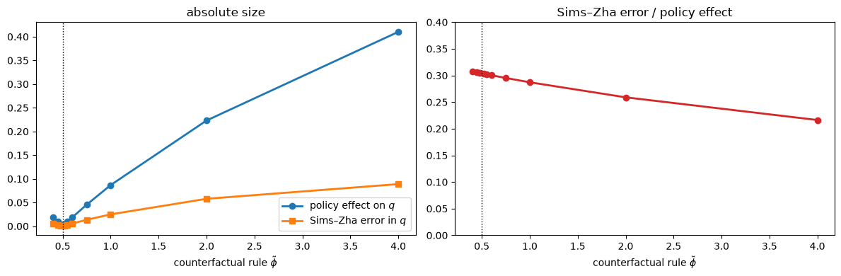
Fig. 29.5 Sims–Zha error for modest interventions#
As the intervention becomes more modest, the Sims–Zha error shrinks in proportion to the effect of the intervention itself.
For interventions near the baseline rule, the Sims–Zha counterfactual misses roughly 30 percent of the effect on quantity that it is trying to measure.
The reason is that both the effect of the intervention and the Sims–Zha error are first order in \(\tilde\phi - \phi_A\), so their ratio tends to a nonzero constant as the intervention shrinks.
A modest intervention makes the absolute error small and leaves the error relative to the policy effect near 30 percent.
The expectational channel that Sims–Zha omits is a first-order part of how the counterfactual rule works: it does not become negligible relative to the other channels as the rule change becomes small.
The Sims–Zha path does correctly answer a different question: what happens if the government repeatedly surprises agents who go on believing that the old rule is in force?
Leeper and Zha’s modesty condition is designed to make that the relevant question, by ensuring that agents would not detect the intervention; the answer differs from the effect of a known change in the rule, which is what McKay and Wolf’s construction delivers.
29.5. Model uncertainty and sufficient statistics#
In Induced Priors for Impulse Responses, a structural modeler who believes the model but is unsure of the adjustment costs expresses that uncertainty with the prior \(g_s \sim U[8, 12]\), \(g_d \sim U[0.05, 0.15]\).
That prior induces a prior over the counterfactual response to a demand shock under the rule \(\tilde\phi = 2\).
McKay and Wolf’s econometrician needs no prior over \((g_s, g_d)\): given estimates of \(x_A(\varepsilon)\) and \(\Theta_\nu\) from data generated by the true economy, Proposition 1 delivers the true counterfactual exactly.
In the language of McKay and Wolf, impulse responses to policy shocks, together with \(x_A(\varepsilon)\), are sufficient statistics for policy counterfactuals: every model in their class that matches those impulse responses implies the same counterfactual.
def fan(ax, paths, color, label, alpha=0.25):
    "Plot the 5-95 percentile band and the median of paths (draws x horizons)."
    lo, med, hi = np.percentile(paths, [5, 50, 95], axis=0)
    h = np.arange(paths.shape[1])
    ax.fill_between(h, lo, hi, color=color, alpha=alpha, lw=0)
    ax.plot(h, med, color=color, lw=2, label=label)

rng = np.random.default_rng(1234)
n_draws = 200
base_draws, cf_draws, sz_ratio_draws = [], [], []
for _ in range(n_draws):
    g_s_i, g_d_i = rng.uniform(8, 12), rng.uniform(0.05, 0.15)
    M_inv_i = system_inverse(g_s_i, g_d_i, φ_A)
    x_A_i = M_inv_i @ forcing(1)
    x_cf_i = np.linalg.solve(np.vstack([private_block(g_s_i, g_d_i), rule_block(φ_new)]),
                             forcing(1))
    x_sz_i, _ = sims_zha(M_inv_i, x_A_i, φ_new)
    base_draws.append(np.concatenate(split(x_A_i)[:2]))
    cf_draws.append(np.concatenate(split(x_cf_i)[:2]))
    sz_ratio_draws.append(np.abs(split(x_sz_i)[0] - split(x_cf_i)[0]).max()
                          / np.abs(split(x_cf_i)[0] - split(x_A_i)[0]).max())
base_draws, cf_draws = np.array(base_draws), np.array(cf_draws)

fig, axes = plt.subplots(1, 2, figsize=(12, 4))
for i, ax in enumerate(axes):
    fan(ax, base_draws[:, i * T:i * T + H_plot], 'C7',
        f"induced prior, baseline rule $\\phi = {φ_A}$")
    fan(ax, cf_draws[:, i * T:i * T + H_plot], 'C1',
        f"induced prior, counterfactual rule $\\tilde\\phi = {φ_new}$")
    ax.plot(split(x_mw)[i][:H_plot], 'C0o', ms=4,
            label="McKay–Wolf, from the true economy's impulse responses")
    ax.axhline(0, color='k', lw=0.5)
    ax.set_title(f"{names[i]}, demand shock")
    ax.set_xlabel("periods")
axes[0].legend(fontsize=8)
plt.tight_layout()
plt.show()

print(f"Sims–Zha error / policy effect on q across the prior: "
      f"[{min(sz_ratio_draws):.2f}, {max(sz_ratio_draws):.2f}]")
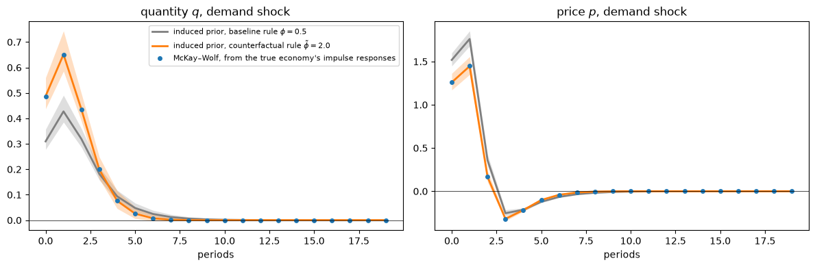
Fig. 29.6 Induced prior versus sufficient statistics#
Sims–Zha error / policy effect on q across the prior: [0.24, 0.28]
The structural modeler’s counterfactual band reflects uncertainty about \((g_s, g_d)\) that, in this exercise, never gets resolved.
The gray band shows that much of this uncertainty is already present in the modeler’s beliefs about how the economy responds under the baseline rule.
The McKay–Wolf econometrician replaces that uncertainty with measurement: given the impulse responses, the counterfactual follows without any parametric model of the private sector.
The Sims–Zha error, meanwhile, is a robust feature of the model: across the whole prior, it misses about a quarter of the policy effect on quantity.
The comparison flatters McKay and Wolf, however, because their econometrician sees population impulse responses while the modeler sees nothing.
A modeler who believes the model and sees the same baseline response \(x_A(\varepsilon)\) can estimate the parameters from it.
We give the modeler the responses of quantity and price to the demand shock under the baseline rule, for 40 periods, and fit two models by least squares: the true one, with \((h_s, g_s, g_d)\) unknown, and one in which demand is static (\(g_d = 0\)).
The modeler also takes as known everything else in the model: \(h_d\), \(a(L)\), \(\beta\), the process \(\sigma_d B_d(L)\) for the demand shock, and the baseline rule \(\phi_A\); McKay and Wolf’s econometrician needs none of these.
def baseline_residuals(θ, static=False):
    "Gap between a model's response to the demand shock under the baseline rule and x_A."
    h_s_, g_s_, g_d_ = (θ[0], θ[1], 0.0) if static else θ
    x_model = np.linalg.solve(np.vstack([private_block(g_s_, g_d_, h_s=h_s_), rule_block(φ_A)]),
                              forcing(1))
    return np.concatenate([(split(x_model)[i] - split(x_A)[i])[:40] for i in range(2)])

peak_A = max(np.abs(split(x_A)[i][:40]).max() for i in range(2))
for label, static, θ0 in [("true model", False, [0.5, 8.0, 0.08]), ("static demand", True, [0.5, 8.0])]:
    fit = least_squares(baseline_residuals, θ0, args=(static,), bounds=(0.0, 100.0))
    h_s_, g_s_, g_d_ = (fit.x[0], fit.x[1], 0.0) if static else fit.x
    x_cf = np.linalg.solve(np.vstack([private_block(g_s_, g_d_, h_s=h_s_), rule_block(φ_new)]),
                           forcing(1))
    err = [np.abs(split(x_cf)[i] - split(x_true)[i]).max() / np.abs(split(x_true)[i]).max()
           for i in range(2)]
    print(f"{label:13s}: estimates {np.round(fit.x, 3)}, fit error {np.abs(fit.fun).max() / peak_A:.3f}, "
          f"counterfactual error q {err[0]:.3f}, p {err[1]:.3f}")
true model   : estimates [ 1.  10.   0.1], fit error 0.000, counterfactual error q 0.000, p 0.000
static demand: estimates [1.043 8.274], fit error 0.064, counterfactual error q 0.308, p 0.074
Within the true model, the baseline response pins down all three parameters, and the modeler’s counterfactual is exact too.
The static-demand model matches the baseline response to within about 6 percent of its peak, yet it misses the counterfactual by 31 percent for quantity.
So, given population responses, a correctly specified model does as well as McKay and Wolf; their advantage is robustness to misspecification: their counterfactual does not depend on which model of the private sector is right.
(In Exercise 28.3 of Induced Priors for Impulse Responses, a modeler learns the parameters from autocovariances instead.)
When do we need a model? returns to this tradeoff when the measured impulse responses are incomplete.
29.6. Measuring the sufficient statistics#
So far the econometrician has known \(x_A(\varepsilon)\) and \(\Theta_\nu\) exactly, at every horizon.
This section asks what she can do with less: evidence on a few policy shocks, data generated under a different rule, and a model fitted to the evidence.
29.6.1. Limited evidence on policy shocks#
McKay and Wolf’s exact result requires the effects of news shocks at every horizon.
In practice an econometrician has evidence on only a few distinct policy shocks, and McKay and Wolf propose choosing the date-0 combination of the available shocks that enforces the counterfactual rule as well as possible in a least-squares sense.
Suppose the econometrician knows the effects of a contemporaneous shock and of news shocks about the next \(n - 1\) periods.
This clean menu is an idealization: identified policy shocks in practice, such as the monetary policy shocks of Romer and Romer [2004] or Gertler and Karadi [2015] that McKay and Wolf use, are combinations of surprises and news about several horizons, each tracing out its own path for the policy instrument.
def mw_limited(M_inv_A, x_A, φ_new, n):
    "Least-squares McKay–Wolf counterfactual using news shocks for horizons 0..n-1."
    Ω = M_inv_A[:, 2 * T:2 * T + n]
    R_new = rule_block(φ_new)
    weights, *_ = np.linalg.lstsq(R_new @ Ω, -R_new @ x_A, rcond=None)
    return x_A + Ω @ weights

ns = np.arange(1, 16)
errors = np.array([[np.abs(split(mw_limited(M_inv_A, x_A, φ_new, n))[i]
                           - split(x_true)[i]).max()
                    / np.abs(split(x_true)[i]).max() for i in range(2)]
                   for n in ns])

fig, ax = plt.subplots()
ax.semilogy(ns, errors[:, 0], 'o-', lw=2, label="quantity")
ax.semilogy(ns, errors[:, 1], 's-', lw=2, label="price")
ax.set_xlabel("number of distinct policy shocks $n$ (news horizons $0, \\ldots, n-1$)")
ax.set_ylabel("max relative error")
ax.legend()
plt.tight_layout()
plt.show()
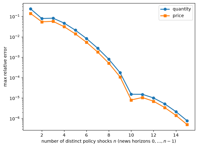
Fig. 29.7 Counterfactuals from limited policy evidence#
Apart from a small step back at \(n = 3\), the error falls quickly as evidence on more distinct policy shocks becomes available: with \(n = 10\) distinct shocks it is below 0.01 percent.
29.6.2. The baseline rule does not matter#
The columns of \(\Theta_\nu\) are responses to shocks to the baseline rule, and they depend on that rule.
What the counterfactual uses, however, is only the path of the tax that each shock produces and that path’s effects on quantity and price.
Define \(\Theta_{(q,p),\tau} = \Theta_{(q,p),\nu} \Theta_{\tau,\nu}^{-1}\), where \(\Theta_{(q,p),\nu}\) and \(\Theta_{\tau,\nu}\) are the quantity-and-price rows and the tax rows of \(\Theta_\nu\).
Column \(\ell\) of \(\Theta_{(q,p),\tau}\) is the response of quantity and price to a path of the tax that rises by one unit at date \(\ell\) and is otherwise zero, known at date 0.
These effects of tax paths are determined by the private sector’s equations (29.1)–(29.2) alone, so they are the same whatever rule generated the data.
Caravello et al. [2026] call policy effects of this kind portable across regimes, and they explain them with an analogy that fits our market exactly:
The intuition echoes insights from the analysis of simple static models of demand and supply: to predict to first order the effect on prices of the quantity demanded changing to some hypothetical level, all we need to know is (i) the initial outcomes plus (ii) the slope of the supply function, and not the slope of demand, nor the actual shocks to demand or supply that generated the observed outcomes.
To map the analogy into our market, note that “supply” and “demand” in the quotation are not our supply and demand.
Their demand curve, the one that shifts, is our tax rule.
Their supply curve, whose slope we need, is the private sector as a whole: our open-loop supply and demand curves (29.1)–(29.2) together, which determine how quantity and price respond to a path of the tax.
Their shocks are our non-policy shocks \(\varepsilon\), which the econometrician need not identify beyond the baseline paths \(x_A(\varepsilon)\).
We compute \(\Theta_{(q,p),\tau}\) from data generated under three different rules and compare it with the effects that the private sector’s equations imply directly.
def tax_effects(g_s_=g_s, g_d_=g_d, h_s_=h_s, m=1.0):
    """
    Θ_(q,p),τ: paths of (q, p) caused by a path of the tax known at date 0, from the
    private sector's equations alone.  Suppliers scale their forecasts of next period's
    quantity by m (m = 1 is rational expectations).
    """
    H = private_block(g_s_, g_d_, h_s=h_s_)
    H[np.arange(T - 1), np.arange(1, T)] *= m       # the supply curve's term in E_t q_(t+1)
    return -np.linalg.solve(H[:, :2 * T], H[:, 2 * T:])

def cf_from_tax_effects(Θ_qpτ_, x_base, φ_new):
    "Counterfactual paths under τ = -φ_new p, from baseline paths and the effects of tax paths."
    q_b, p_b, τ_b = split(x_base)
    P = Θ_qpτ_[T:]                                  # effects of tax paths on the price
    τ_new = np.linalg.solve(np.eye(T) + φ_new * P, φ_new * (P @ τ_b - p_b))
    return np.concatenate([np.concatenate([q_b, p_b]) + Θ_qpτ_ @ (τ_new - τ_b), τ_new])

Θ_qpτ = tax_effects()
for φ in [-0.5, 0.5, 2.0]:
    M_inv_φ = system_inverse(g_s, g_d, φ)
    Θ_φ = M_inv_φ[:, 2 * T:]
    from_data = Θ_φ[:2 * T] @ np.linalg.inv(Θ_φ[2 * T:])
    x_cf = cf_from_tax_effects(from_data, M_inv_φ @ forcing(1), φ_new)
    print(f"data generated under φ = {φ:4}: max |Θ_(q,p),τ from data - from the private sector| = "
          f"{np.abs(from_data - Θ_qpτ).max():.1e};  counterfactual error {np.abs(x_cf - x_true).max():.1e}")
data generated under φ = -0.5: max |Θ_(q,p),τ from data - from the private sector| = 4.2e-16;  counterfactual error 3.1e-15
data generated under φ =  0.5: max |Θ_(q,p),τ from data - from the private sector| = 1.8e-16;  counterfactual error 1.3e-15
data generated under φ =  2.0: max |Θ_(q,p),τ from data - from the private sector| = 7.8e-16;  counterfactual error 4.4e-16
Whichever rule generated the data, the effects of tax paths are the same, and so is the counterfactual built from them.
The baseline rule matters only through the baseline paths \(x_A(\varepsilon)\), which the econometrician observes.
29.6.3. When do we need a model?#
Caravello et al. [2026] argue that the available evidence on policy shocks mostly concerns short-lived changes in the policy instrument, and that the effects of more persistent or delayed changes must come from somewhere else.
Their proposal is a hybrid: fit a model of the private sector to the evidence on policy shocks, as in the impulse-response matching of Christiano et al. [2005], and then use the fitted model’s effects of all tax paths in the counterfactual.
Where the evidence speaks, the fitted model agrees with it; elsewhere, the model extrapolates.
Suppose the econometrician has evidence on two policy shocks: a surprise, \(\nu_{0,0} = 1\), and a shock that announces at date 0 the deviations \(\nu_{\ell,0} = 0.6^\ell\) from the rule.
Under the baseline rule, the tax paths that they produce are short-lived: \((0.96, -0.03, -0.02, \ldots)\) and \((0.94, 0.52, 0.29, 0.16, \ldots)\).
With only these two shocks, McKay and Wolf’s least-squares construction approximates the counterfactual poorly.
The econometrician instead estimates the parameters of a model of the private sector by matching the responses of quantity and price to the two observed tax paths, and then uses the fitted model’s \(\Theta_{(q,p),\tau}\) in the counterfactual.
Matching uses the private sector’s equations only, so the econometrician need not know the baseline rule.
We try three models: the true one with unknown parameters, one in which demand is static (\(g_d = 0\)), and one in which suppliers form “behavioral” expectations, scaling their forecasts of next period’s quantity by \(m = 0.8\), as in the cognitive discounting of Gabaix [2020].
evidence_shocks = [np.eye(T)[0], 0.6 ** np.arange(T)]      # a surprise and a decaying shock path
evidence = [Θ_ν @ v for v in evidence_shocks]               # observed responses of (q, p, τ)
H_fit = 40                                                  # horizons used in the matching

Ω_two = np.column_stack(evidence)
w_two, *_ = np.linalg.lstsq(rule_block(φ_new) @ Ω_two, -rule_block(φ_new) @ x_A, rcond=None)
x_two = x_A + Ω_two @ w_two

def cf_error(x):
    "Largest error in (q, p) relative to the peak of the true counterfactual."
    return [np.abs(split(x)[i] - split(x_true)[i]).max() / np.abs(split(x_true)[i]).max()
            for i in range(2)]

def matching_residuals(model):
    "Residuals from matching the responses of (q, p) to the observed tax paths."
    def residuals(θ):
        Θ_m = model(θ)
        out = []
        for x in evidence:
            q, p, τ = split(x)
            out.append((Θ_m @ τ - np.concatenate([q, p]))[np.r_[0:H_fit, T:T + H_fit]])
        return np.concatenate(out)
    return residuals

peak = max(np.abs(np.concatenate(split(x)[:2])).max() for x in evidence)
models = {
    "true model, (h_s, g_s, g_d) estimated": (lambda θ: tax_effects(θ[1], θ[2], h_s_=θ[0]), [0.5, 5.0, 0.5]),
    "static demand, (h_s, g_s) estimated":   (lambda θ: tax_effects(θ[1], 0.0, h_s_=θ[0]), [0.5, 5.0]),
    "behavioral suppliers, m = 0.8":         (lambda θ: tax_effects(θ[1], θ[2], h_s_=θ[0], m=0.8),
                                              [0.5, 5.0, 0.5]),
}
print(f"{'method':40s}  {'estimates':24s}  {'fit error':10s}  counterfactual error")
print(f"{'least squares on the two shocks':40s}  {'':24s}  {'':10s}  "
      f"q {cf_error(x_two)[0]:.3f}  p {cf_error(x_two)[1]:.3f}")
fitted = {}
for name, (model, θ0) in models.items():
    fit = least_squares(matching_residuals(model), θ0, bounds=(0.0, 100.0))
    fitted[name] = model(fit.x)
    err = cf_error(cf_from_tax_effects(fitted[name], x_A, φ_new))
    print(f"{name:40s}  {str(np.round(fit.x, 3)):24s}  {np.abs(fit.fun).max() / peak:10.3f}  "
          f"q {err[0]:.3f}  p {err[1]:.3f}")
method                                    estimates                 fit error   counterfactual error
least squares on the two shocks                                                 q 0.147  p 0.102
true model, (h_s, g_s, g_d) estimated     [ 1.  10.   0.1]               0.000  q 0.000  p 0.000
static demand, (h_s, g_s) estimated       [0.92  8.295]                  0.193  q 0.104  p 0.021
behavioral suppliers, m = 0.8             [0.    8.763 0.103]            0.061  q 0.020  p 0.014
With only two short-lived policy shocks, least squares misses the counterfactual by about 15 percent for quantity, against 8 percent with the surprise and the one-period news shock of Limited evidence on policy shocks.
The counterfactual calls for large negative deviations from the baseline rule at dates 0 and 1 and small ones afterward, as the policy shocks in Fig. 29.3 show; news about date 1 can supply them, but the decaying shock cannot deliver a deviation at date 1 without also delivering deviations at later dates.
The true model, fitted to the same two responses, recovers its parameters and the counterfactual exactly: the evidence pins down the model, and the model supplies the effects of all other tax paths.
The two misspecified models cannot match the evidence exactly, but both beat least squares, and their counterfactual errors are well below their misfit.
The static-demand model misses the evidence by 19 percent of its peak and the counterfactual by 10 percent for quantity; the behavioral model misses them by 6 and 2 percent.
(The behavioral fit puts \(h_s\) at its lower bound of zero.)
The counterfactual with \(\tilde\phi = 2\) relies mostly on short-lived tax changes, which the evidence covers.
The models disagree more where the evidence is silent.
The next figure shows the response of quantity to news, received at date 0, of a one-unit tax at date 8, and the code reports how well each fitted model predicts the effect of a tax of one unit at dates 8 through 12, announced at date 0.
τ_announced = np.zeros(T)
τ_announced[8:13] = 1.0
effect_true = Θ_qpτ @ τ_announced

fig, ax = plt.subplots()
ax.plot(Θ_qpτ[:H_plot, 8], 'k', lw=2, label="true effect")
for (name, Θ_m), style in zip(fitted.items(), ['ko', 'C0--', 'C3-.']):
    ax.plot(Θ_m[:H_plot, 8], style, lw=2, ms=4, label=name)
    effect = Θ_m @ τ_announced
    err = [np.abs(effect[b * T:(b + 1) * T] - effect_true[b * T:(b + 1) * T]).max()
           / np.abs(effect_true[b * T:(b + 1) * T]).max() for b in range(2)]
    print(f"{name:40s}: error for the announced tax at dates 8-12, q {err[0]:.3f}, p {err[1]:.3f}")
ax.axhline(0, color='k', lw=0.5)
ax.axvline(8, color='k', ls=':', lw=1)
ax.set_xlabel("periods")
ax.set_ylabel("response of $q$ to a unit tax at date 8")
ax.legend(fontsize=8)
plt.tight_layout()
plt.show()
true model, (h_s, g_s, g_d) estimated   : error for the announced tax at dates 8-12, q 0.000, p 0.000
static demand, (h_s, g_s) estimated     : error for the announced tax at dates 8-12, q 0.369, p 0.196
behavioral suppliers, m = 0.8           : error for the announced tax at dates 8-12, q 0.178, p 0.169
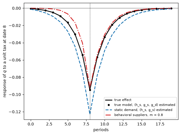
Fig. 29.8 Fitted models and news about a distant tax#
Suppliers in the behavioral model discount the future, so they respond much less in advance; the static-demand model responds more.
For the announced tax at dates 8 through 12, the misspecified models miss the response of quantity by 37 and 18 percent, several times their errors for the counterfactual rule.
Caravello et al. [2026] find a related pattern for monetary policy.
Behavioral frictions in price setters’ expectations, like our behavioral suppliers, change how models fitted to the same evidence on short-lived interest-rate changes extrapolate to distant ones, whereas household heterogeneity barely does; in their application all these models fit the evidence about equally well, while here both misspecified models miss it.
Evidence of another kind can do some of the model’s work.
Suppose the econometrician has also observed the market under a second rule and measured the response to a demand shock there.
As Policy Regimes and the Lucas Critique shows, following Manuel and Wolf [2026], the difference between the responses to the same non-policy shock under two rules is the effect of a path of the tax, so it can serve as a third column alongside the two policy shocks.
for φ_other in [0.0, 1.0]:
    comparison = system_inverse(g_s, g_d, φ_other) @ forcing(1) - x_A
    Ω_three = np.column_stack([Ω_two, comparison])
    w_three, *_ = np.linalg.lstsq(rule_block(φ_new) @ Ω_three, -rule_block(φ_new) @ x_A, rcond=None)
    err = cf_error(x_A + Ω_three @ w_three)
    print(f"two policy shocks plus the comparison with φ = {φ_other}: "
          f"counterfactual error q {err[0]:.4f}, p {err[1]:.4f}")
two policy shocks plus the comparison with φ = 0.0: counterfactual error q 0.0182, p 0.0132
two policy shocks plus the comparison with φ = 1.0: counterfactual error q 0.0085, p 0.0060
Adding the comparison with laissez-faire cuts the least-squares error from 15 to 1.8 percent for quantity, and the comparison with \(\phi = 1\) cuts it to 0.85 percent.
The comparison with laissez-faire contributes, with its sign reversed, the baseline rule’s own response of the tax to a demand shock, a path with the shape that the counterfactual needs.
29.7. Optimal policy from impulse responses#
McKay and Wolf’s sufficient statistics deliver optimal policy as well as the outcomes of given rules.
Three exercises at the end of the lecture work this out for a policymaker who, after a demand shock, minimizes \(\frac12 \sum_t \beta^t (p_t^2 + \lambda q_t^2)\).
This loss is a stand-in for a stabilization mandate, like the inflation and output objectives of McKay and Wolf’s monetary application, not a measure of welfare.
In this market the untaxed equilibrium maximizes the sum of demanders’ and suppliers’ objectives (Dynamic Supply and Demand Curves), so any tax lowers total surplus, counting the tax revenue, and a planner who maximized surplus would set \(\tau_t = 0\).
Exercise 29.1 computes the optimal plan under commitment, McKay and Wolf’s Proposition 2, as a least-squares problem in \(\Theta_\nu\), and verifies their targeting rule; the plan subsidizes the good heavily while the demand shock raises its price and then taxes it.
Exercise 29.2 shows that the plan is time inconsistent, as are the Ramsey plans of Time Inconsistency of Ramsey Plans and Stackelberg Plans, but only slightly: a policymaker who re-optimizes later raises taxes that the plan held down only to shape earlier expectations.
Exercise 29.3 computes optimal policy under discretion with the algorithm of Hebden and Winkler [2026]: each policymaker chooses the current tax, taking as given the rules that its successors will follow; discretion raises the loss by less than one percent in this market.
29.8. McKay and Wolf and dynamic programming squared#
Several lectures in this series — the “dynamic programming squared” lectures — pursue a different response to the Lucas critique: they model the government as an optimizing agent and ask which policies it would choose and which it could credibly promise.
29.8.1. Rule-based scenario analysis#
McKay and Wolf describe their thought experiment, in which a monetary policy rule links the interest rate \(i\) to inflation \(\pi\):
Note that this thought experiment supposes that the private sector perfectly understands the change in rule: the new relationship between \(i\) and \(\pi\) holds for all \(t \geq 0\).
Their counterfactual is a scenario: a government announces a rule at date 0, private agents believe it and expect it to hold forever, and the analyst computes outcomes under rational expectations.
Because the economy is linear, a rule is equivalent, shock by shock, to one path of the policy instrument; a rule counterfactual is a family of path scenarios, one for each history of shocks, and a peg or a zeroing-out counterfactual is a single path.
Lucas [1976] proposed this kind of experiment: compare outcomes under alternative rules, each a permanent change that private agents understand.
McKay and Wolf carry out Lucas’s experiment with measured impulse responses in place of an estimated model of the private sector.
Sargent and Wallace [1976] and Sims [1982] questioned the experiment.
If rules can change, rational agents assign probabilities to changes before they occur, and the historical data already reflect those probabilities.
A rule change that agents did not anticipate before date 0 and believe completely after date 0 lies outside the stochastic process that generated the data.
The construction also requires that the instrument path implementing the new rule lie in the span of paths traced out by historical policy shocks; a rule never followed in the sample can satisfy that requirement, but the date-0 news shocks that implement it may be large by historical standards, in which case Leeper and Zha’s modesty condition fails.
The scenario does not explain why a government would adopt the rule, keep it, or be believed.
The dynamic programming squared lectures address those questions.
Caravello et al. [2026] show that McKay and Wolf’s sufficient statistics also deliver outcomes when the counterfactual is itself a known stochastic process for rules, for example a reform that may be reversed.
The new process, however, is still announced at date 0 and believed: the construction applies Lucas’s experiment to a process for rules rather than to a single rule.
29.8.2. The same constraint, measured or modeled#
In Time Inconsistency of Ramsey Plans, a perfect-foresight Cagan demand for money implies that the rate of inflation,
depends on the entire future path of money growth \(\{\mu_{t+j}\}\).
Inflation summarizes how future policy affects today’s real balances.
In Stackelberg Plans, a Stackelberg follower’s Euler equations are part of the law of motion that the Stackelberg leader faces when it chooses its plan.
In Optimal Taxation with State-Contingent Debt, the household’s first-order conditions collapse into an implementability constraint that restricts the allocations a Ramsey planner can implement with distorting taxes.
In each case, private decisions depend on the whole expected path of a policy instrument, and a policymaker who chooses that path takes the dependence into account.
Our Euler equations (29.1)–(29.2) are the corresponding constraint, and McKay and Wolf’s key assumption is that they are the only channel through which policy matters.
The matrix \(\Theta_\nu\) of responses to contemporaneous and news shocks is then an empirical counterpart of the constraint that the planners of those lectures take from a model: it tells us which paths of \((q_t, p_t)\) a policymaker can implement by choosing a path for the tax.
29.8.3. Commitment, discretion, and credibility#
McKay and Wolf’s Proposition 2 is a Ramsey or Stackelberg problem written in sequence space, and like the plans of Time Inconsistency of Ramsey Plans, Stackelberg Plans, and Optimal Taxation with State-Contingent Debt its solution is time inconsistent (Optimal policy from impulse responses).
Stackelberg Plans and Optimal Taxation with State-Contingent Debt implement such a plan recursively by handing each continuation planner, as a state variable, the forward-looking variable that its predecessors promised — the follower’s decision in Stackelberg Plans, marginal-utility-weighted government debt in Optimal Taxation with State-Contingent Debt.
Hebden and Winkler [2026] show that the commitment plan can be implemented in sequence space by applying the targeting rule to revisions of forecasts at each date, with past promises carried in the previous period’s expected path, a counterpart of the recursive contracts of Marcet and Marimon [2019]; they note that this implements the date-0 plan rather than a plan chosen from a timeless perspective.
Their discretionary equilibrium, computed in Exercise 29.3, is the sequence-space counterpart of the Markov perfect governments of Time Inconsistency of Ramsey Plans.
Sustainable Plans for a Calvo Model studies sustainable plans, in which a sequence of policymakers each choose policy for one period and a plan is sustained by the private sector’s expectation that a deviation would trigger a worse continuation plan [Abreu, 1988, Chari and Kehoe, 1990, Stokey, 1989].
That theory makes credibility an equilibrium outcome, where McKay and Wolf’s scenario assumes it, and it treats a deviation from expected policy as an event that changes beliefs about future policy.
If measured policy shocks are deviations of that kind, their estimated effects combine the effect of the instrument path with a revision of beliefs about the rule, and the premise of Proposition 1 fails; Leeper and Zha’s modesty condition rules this out.
29.8.4. Endogenous policy regimes and institutional counterfactuals#
Accounting for Monetary and Fiscal Policy studies a model of Bocola et al. [2026] in which a government that cannot fully commit delegates monetary policy to a central bank with an inflation mandate but may override the mandate when it needs revenue, so that the economy switches endogenously between monetary-dominant and fiscal-dominant regimes.
Endogenous switching is not by itself the obstacle: Manuel and Wolf [2026] allow policy that switches with the state of the economy, and Caravello et al. [2026] allow rules that switch with exogenous probabilities and, reinterpreted, a lower bound on the instrument that binds for a stochastic number of periods, as long as the private sector’s equations stay linear and depend on policy only through the instrument.
Two features put the economy of Accounting for Monetary and Fiscal Policy outside these methods.
Private demand for money depends on the probability that the mandate will be honored, not only on the expected path of the instrument, a nonlinearity that breaks the certainty equivalence behind McKay and Wolf’s expected paths.
And its central counterfactual — setting the cost of overriding the mandate to zero — changes the institutions that determine how policy is chosen, not the rule that policy follows, a question that calls for a structural model of the policymaker.
29.8.5. What the method takes for granted#
McKay and Wolf’s counterfactuals are exact under seven assumptions, several of which the dynamic programming squared lectures relax.
The private sector’s behavior is linear and depends on policy only through the expected path of the instrument.
The counterfactual rule is credible: announced at date 0, understood, believed, and kept; Caravello et al. [2026] allow the counterfactual to be a stochastic process of rules, but the process itself must be announced at date 0 and believed.
Measured policy shocks change the instrument path without changing beliefs about the rule.
The policy rule is a primitive chosen by the analyst, not the outcome of choices by a government that may be unable to commit.
The question concerns rules, not the institutions that shape how rules are chosen.
The baseline rule delivers a unique equilibrium; McKay and Wolf also assume that the counterfactual rule does, but Caravello et al. [2026] show that when it does not, the same sufficient statistics deliver every counterfactual equilibrium, so that the analyst must add a criterion for selecting one; the theory of sustainable plans, with its many credible plans, likewise warns that a policy environment need not pin down one outcome.
The econometrician knows \(x_A(\varepsilon)\) and the responses to policy shocks at all horizons; with less, she must approximate or lean on a model (Measuring the sufficient statistics), and estimating those responses raises questions of identification and invertibility.
Our market satisfies the first assumption, our computations impose the next three by construction, and every rule we study satisfies the sixth (Price stabilization as more flexible supply).
Within these assumptions, McKay and Wolf replace a model of the private sector with measurements; the dynamic programming squared lectures, in turn, replace an assumed policy rule with a model of the policymaker.
29.9. Beyond this lecture#
29.9.1. Estimating the sufficient statistics#
We have assumed that the econometrician can estimate the impulse responses that McKay and Wolf’s method uses, but in this market the supply shock is not fundamental for prices and quantities, as in Dynamic Supply and Demand Curves and Induced Priors for Impulse Responses.
Invertibility and Policy Counterfactuals sorts estimation procedures by whether they need invertibility: local projections on an instrument recover the supply-shock response that no rotation of VAR innovations can, whether the supply shock is fundamental depends on the policy rule, and McKay and Wolf’s route to counterfactual second moments through VAR innovations makes only a tiny error here, partly because supply shocks account for less than half a percent of the variance of quantity.
That lecture also shows that, in samples of realistic length, local projections on an instrument are noisy, a practical cost of their robustness to non-invertibility.
29.9.2. When policy regimes switch#
Policy Regimes and the Lucas Critique lets the tax rule switch between laissez-faire and price stabilization according to a Markov chain that private agents know, in a version of the market with static demand whose equilibrium solves a Markov jump linear quadratic problem of the kind studied in Markov Jump Linear Quadratic Dynamic Programming.
McKay and Wolf’s construction recovers outcomes under a permanent rule from data generated by switching regimes.
Written on the tree of regime histories, as Caravello et al. [2026] propose, it also delivers a reform that agents expect may be reversed: with a probability 0.2 of reversal each period, the response of quantity one period after a demand shock is about 7 percent smaller than under a permanent reform.
Following Manuel and Wolf [2026], regime switches in the data can also take the place of policy shocks, although in samples of a few hundred periods the evidence they deliver is imprecise.
29.9.3. Rules with many equilibria#
Policy Counterfactuals in a New Keynesian Economy turns to a New Keynesian economy, in which, unlike any rule in our market, an interest-rate peg admits many equilibria, and shows how McKay and Wolf’s sufficient statistics deliver all of them and how an assumption about monetary or fiscal dominance selects one.
29.10. Summary#
The market with a tax fits McKay and Wolf’s framework, and their key assumption is the invariance of the open-loop dynamic supply and demand curves of Dynamic Supply and Demand Curves.
In this market:
Impulse responses to contemporaneous and news tax shocks under one rule deliver the exact response to supply and demand shocks under another rule.
The Sims–Zha method, which uses only contemporaneous surprises, makes errors in quantity that, beyond very small adjustment costs, grow with how forward-looking suppliers are.
Making the intervention more modest shrinks the Sims–Zha error only in proportion to the policy effect itself: near the baseline rule it still misses about 30 percent of the effect on quantity.
With evidence on only a few distinct policy shocks, McKay and Wolf’s least-squares approximation misses the counterfactual by about 8 percent with two shocks, by less than 1 percent with six, and by less than 0.01 percent with ten.
Impulse responses to policy shocks, together with the baseline responses to the shock of interest, are sufficient statistics for the counterfactual: every model in McKay and Wolf’s class that matches them implies the same counterfactual, whereas a modeler who fits a misspecified model to the baseline response alone can miss the counterfactual badly.
The effects of tax paths are the same whatever rule generated the data.
A model fitted to evidence on two short-lived policy shocks recovers the counterfactual exactly when it is the right model; when it is not, it still beats least squares on the same two shocks, although it extrapolates poorly to distant tax changes; adding the response to a demand shock under a second rule cuts the least-squares error to 2 percent or less.
A price-stabilizing tax rule is observationally equivalent to more flexible suppliers, a compact form of the Lucas critique in this market.
The same sufficient statistics deliver optimal policy under commitment and under discretion; in this market, commitment improves on discretion only slightly.
Finally, McKay and Wolf’s counterfactual is rule-based scenario analysis: a rule announced at date 0 and believed forever.
The lectures listed in Beyond this lecture take up how the sufficient statistics can be estimated, rule changes that agents expect may be reversed, and counterfactual rules that admit many equilibria.
29.11. Exercises#
Exercise 29.1
McKay and Wolf’s Proposition 2 shows that impulse responses to policy shocks also suffice to compute optimal policy for a given loss function.
Consider a policymaker who, after a demand shock, wants to minimize
by choosing the date-0 policy shocks \(\nu\).
Using only \(x_A(\varepsilon)\) and \(\Theta_\nu\) under the baseline rule, compute the optimal responses of \((q_t, p_t, \tau_t)\) for \(\lambda = 0.1\) and \(\lambda = 1\).
Verify that the optimal allocation satisfies McKay and Wolf’s targeting rule \(\Theta_{p,\nu}^\top \mathcal{B} p + \lambda\, \Theta_{q,\nu}^\top \mathcal{B} q = 0\), where \(\mathcal{B} = \mathrm{diag}(1, \beta, \beta^2, \ldots)\) and \(\Theta_{p,\nu}, \Theta_{q,\nu}\) are the price and quantity rows of \(\Theta_\nu\).
Solution
The loss is a weighted sum of squares of \(x_A + \Theta_\nu \nu\), and the optimal \(\nu\) solves a least-squares problem.
disc = β ** np.arange(T)                  # discount weights, the diagonal of 𝓑
Θ_q, Θ_p = Θ_ν[:T], Θ_ν[T:2 * T]

def optimal_plan(x_base, Θ, λ, start=0):
    """
    Choose the policy shocks in the columns of Θ to minimize
    sum_{t >= start} β^(t-start) (p_t^2 + λ q_t^2), starting from the path x_base.
    """
    w = np.sqrt(disc[:T - start])
    q_b, p_b, _ = split(x_base)
    A_ls = np.vstack([w[:, None] * Θ[T + start:2 * T],
                      np.sqrt(λ) * w[:, None] * Θ[start:T]])
    b_ls = -np.concatenate([w * p_b[start:], np.sqrt(λ) * w * q_b[start:]])
    ν_opt, *_ = np.linalg.lstsq(A_ls, b_ls, rcond=None)
    return x_base + Θ @ ν_opt

fig, axes = plt.subplots(1, 3, figsize=(14, 4))
for i in range(3):
    axes[i].plot(split(x_A)[i][:H_plot], 'k:', lw=2, label="baseline rule")
for λ, color in [(0.1, 'C0'), (1.0, 'C1')]:
    x_opt = optimal_plan(x_A, Θ_ν, λ)
    q_o, p_o, τ_o = split(x_opt)
    foc = Θ_p.T @ (disc * p_o) + λ * Θ_q.T @ (disc * q_o)
    print(f"λ = {λ}: max |targeting rule| = {np.abs(foc).max():.1e}")
    for i in range(3):
        axes[i].plot(split(x_opt)[i][:H_plot], color=color, lw=2,
                     label=f"optimal, $\\lambda = {λ}$")
for i in range(3):
    axes[i].axhline(0, color='k', lw=0.5)
    axes[i].set_title(f"{names[i]}, demand shock")
    axes[i].set_xlabel("periods")
axes[0].legend()
plt.tight_layout()
plt.show()
λ = 0.1: max |targeting rule| = 6.0e-16
λ = 1.0: max |targeting rule| = 3.3e-16
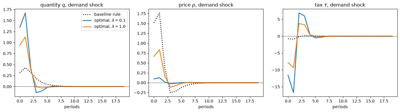
The targeting rule holds to machine precision: it is the first-order condition of the least-squares problem.
A policymaker who cares mostly about the price (\(\lambda = 0.1\)) subsidizes the good heavily when the demand shock raises its price; a larger weight on quantity tempers the subsidy, because the subsidy raises quantity.
The subsidies are large: with \(\lambda = 0.1\) the tax is about \(-11.6\) and \(-16.8\) at dates 0 and 1, against \(-0.8\) and \(-0.9\) under the baseline rule.
They are followed by taxes of about 6.9 and 6.0 at dates 2 and 3, which bring quantity back down quickly as the demand shock fades, so that the price falls much less below normal than under the baseline rule (\(-0.03\) against \(-0.25\) at date 3).
With \(\lambda = 0.1\), a policymaker who chose each date’s tax afresh would set nearly the same taxes, as Exercise 29.3 shows; what commitment adds is a small adjustment of them, made to shape expectations at earlier dates, and Exercise 29.2 shows that this adjustment is time inconsistent.
A loss that also penalized movements in the tax would make these swings smaller; we keep McKay and Wolf’s loss, which does not.
The targeting rule says that the policymaker’s forecasts of its targets must be optimal within the set of forecasts that policy can implement, which is the idea of forecast targeting proposed by Svensson [1997].
The policymaker chooses the optimal plan once and for all at date 0.
The plan works partly through promises about future taxes that shape suppliers’ and demanders’ expectations today.
The plan is a Ramsey plan with commitment — a Stackelberg leader’s plan in the language of Stackelberg Plans — and like the plans in Time Inconsistency of Ramsey Plans, Stackelberg Plans, and Optimal Taxation with State-Contingent Debt it is time inconsistent, as the next exercise shows.
Exercise 29.2
Continue the previous exercise with \(\lambda = 0.1\).
Suppose that the economy follows the date-0 optimal plan through date \(k - 1\), and that at date \(k\) a new policymaker with the same loss function re-optimizes, choosing the policy shocks for dates \(t \ge k\) to minimize \(\frac12 \sum_{t \ge k} \beta^{t-k} (p_t^2 + \lambda q_t^2)\).
The re-optimizing policymaker takes as given everything that happened before date \(k\), including the quantities \(q_{k-1}, \ldots, q_{k-4}\) that enter the Euler equations from date \(k\) on.
Show that for \(k = 1, 2, 4\) the re-optimized path differs from the continuation of the date-0 plan.
Hint: to impose the history, replace the equations for dates \(t < k\) in the stacked system by equations that set \((q_t, p_t, \tau_t)\) equal to their values under the date-0 plan.
Solution
This is the “reborn Stackelberg leader” calculation of Stackelberg Plans, carried out with McKay–Wolf objects.
The re-optimizing policymaker could choose to continue the date-0 plan, which satisfies all the equations from date \(k\) on; if it chooses something else, the date-0 plan is time inconsistent.
λ = 0.1
x_plan = optimal_plan(x_A, Θ_ν, λ)
M_A = np.vstack([private_block(g_s, g_d), rule_block(φ_A)])

def continuation_loss(x, k):
    q, p, _ = split(x)
    return 0.5 * np.sum(disc[:T - k] * (p[k:]**2 + λ * q[k:]**2))

fig, axes = plt.subplots(1, 3, figsize=(14, 4))
for i in range(3):
    axes[i].plot(split(x_plan)[i][:H_plot], 'k', lw=2, label="date-0 plan")
for k, color in [(1, 'C0'), (2, 'C1'), (4, 'C2')]:
    M_k, rhs_k = M_A.copy(), forcing(1)
    for b in range(3):                    # impose the history before date k
        for t in range(k):
            M_k[b * T + t] = 0.0
            M_k[b * T + t, b * T + t] = 1.0
            rhs_k[b * T + t] = x_plan[b * T + t]
    M_k_inv = np.linalg.inv(M_k)
    x_k_base = M_k_inv @ rhs_k            # history, then the baseline rule
    Θ_k = M_k_inv[:, 2 * T:][:, k:]       # policy shocks for dates t >= k
    x_reopt = optimal_plan(x_k_base, Θ_k, λ, start=k)
    gap = [np.abs(split(x_reopt)[i][k:] - split(x_plan)[i][k:]).max() / np.abs(split(x_plan)[i]).max()
           for i in range(3)]
    print(f"k = {k}: max |re-optimized - plan| relative to the plan's peak: q {gap[0]:.3f}, "
          f"p {gap[1]:.3f}, τ {gap[2]:.3f};  continuation loss "
          f"{continuation_loss(x_reopt, k):.4f} vs {continuation_loss(x_plan, k):.4f}")
    print(f"        tax at date {k}: plan {split(x_plan)[2][k]:.2f}, re-optimized {split(x_reopt)[2][k]:.2f}")
    for i in range(3):
        axes[i].plot(np.arange(k, H_plot), split(x_reopt)[i][k:H_plot], '--',
                     color=color, lw=2, label=f"re-optimized at date {k}")
for i in range(3):
    axes[i].axhline(0, color='k', lw=0.5)
    axes[i].set_title(f"{names[i]}, demand shock, $\\lambda = {λ}$")
    axes[i].set_xlabel("periods")
axes[0].legend(fontsize=8)
plt.tight_layout()
plt.show()
k = 1: max |re-optimized - plan| relative to the plan's peak: q 0.005, p 0.084, τ 0.009;  continuation loss 0.1575 vs 0.1576
        tax at date 1: plan -16.76, re-optimized -16.62
k = 2: max |re-optimized - plan| relative to the plan's peak: q 0.010, p 0.167, τ 0.017;  continuation loss 0.0102 vs 0.0106
        tax at date 2: plan 6.88, re-optimized 7.18
k = 4: max |re-optimized - plan| relative to the plan's peak: q 0.003, p 0.039, τ 0.006;  continuation loss 0.0006 vs 0.0007
        tax at date 4: plan 0.48, re-optimized 0.57
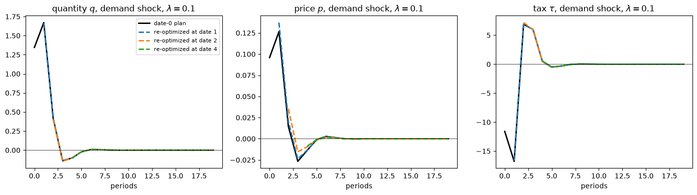
At each date \(k\) the re-optimizing policymaker achieves a lower continuation loss by abandoning the date-0 plan.
The gains are small: at \(k = 1\) the continuation loss falls from 0.1576 to 0.1575.
The departures from the plan are at most 2 percent of the plan’s peak for quantity and the tax, and up to 17 percent for the price, at \(k = 2\).
The date-0 policymaker would not want those departures.
The date-0 plan promised taxes for dates \(t \ge k\) whose purpose was partly to shape expectations at dates before \(k\); once those dates have passed, the promises no longer serve that purpose, and a re-optimizing policymaker wants to break them.
The promises in question are small adjustments, not the large taxes themselves.
At \(k = 2\), the re-optimizing policymaker raises the date-2 tax from 6.88 to 7.18.
The date-0 plan held that tax down because news of a lower tax at date 2 raised supply at date 1, the date at which the demand shock pushes the price up most.
At \(k = 1\), for the same reason, the re-optimizing policymaker cuts the date-1 subsidy from 16.76 to 16.62: part of the planned subsidy was there to raise supply at date 0.
This is the time inconsistency that Time Inconsistency of Ramsey Plans studies in a model of inflation.
A re-optimizing policymaker who honored those promises would continue the date-0 plan, as in the recursive implementations discussed in McKay and Wolf and dynamic programming squared.
Exercise 29.3
Under discretion, the tax at each date is set by a policymaker who takes as given the past and the rules that later policymakers will follow, and who cannot commit to future taxes.
Hebden and Winkler [2026] compute a subgame-perfect equilibrium of this game, which they also describe as Markov perfect, from \(x_A(\varepsilon)\) and \(\Theta_\nu\) alone.
Let \(x^{(h)}\) stack the paths of \((q, p, \tau)\) that are expected at date \(h\), from date \(h\) on, path by path as in the code; let \(F\) shift each path forward one period; and suppose that every policymaker sets policy so that \(\delta\, x^{(h)} = 0\) for some row vector \(\delta\).
A policymaker at date \(h\) who expects her successors to follow \(\delta\) chooses a revision \(\hat\nu\) of the expected policy shocks to minimize \(\frac12 x^{(h)\top} W_\lambda x^{(h)}\) subject to
where \(\bar x^{(h)}\) is the path she inherits and \(W_\lambda = \mathrm{diag}(\lambda \mathcal{B}, \mathcal{B}, 0)\) holds the weights of the loss in Exercise 29.1 on quantity, price, and the tax.
The constraints leave her one degree of freedom, the current tax.
Let \(\zeta\) be the revision that raises the current policy shock by one unit and adjusts later shocks so that her successors’ rules still hold.
Her first-order condition is \(\delta\, x^{(h)} = 0\) with \(\delta = (\Theta_\nu \zeta)^\top W_\lambda\).
Starting from \(\delta = \theta_0^\top W_\lambda\), where \(\theta_0\) is the first column of \(\Theta_\nu\), iterate on the map from \(\delta\) to \(\zeta\) to a new \(\delta\) until it converges.
Compute the discretionary responses to a demand shock for \(\lambda = 0.1\) and \(\lambda = 1\), and compare them and their losses with the commitment plans of Exercise 29.1.
Verify that, when her successors follow \(\delta\), the date-0 policymaker cannot lower her loss by choosing a different current tax.
Solution
Stack the successors’ rules as the rows \(\delta F, \delta F^2, \ldots\) of a matrix \(D\), and split \(\Theta_\nu\) into its first column \(\theta_0\) and the remaining columns \(\Theta_\nu^{+}\).
The revision \(\zeta\) sets the current shock to one and the later shocks to \(-(D \Theta_\nu^{+})^{-1} D\, \theta_0\).
def stack_rules(d):
    "Rows δ F^k, k = 0, ..., T-1: the rule applied to the path expected k periods later."
    D = np.zeros((T, 3 * T))
    D[0] = d
    for k in range(1, T):
        for b in range(3):
            D[k, b * T + 1:(b + 1) * T] = D[k - 1, b * T:(b + 1) * T - 1]
    return D

def loss_weights(λ):
    "The diagonal of W_λ: weights on (q, p, τ)."
    return np.concatenate([λ * disc, disc, np.zeros(T)])

def discretion(λ, tol=1e-14, max_iter=500):
    "Hebden–Winkler rule δ and the discretionary response to a demand shock."
    w = loss_weights(λ)
    θ_0, Θ_plus = Θ_ν[:, 0], Θ_ν[:, 1:]
    d = θ_0 * w
    for it in range(max_iter):
        D_future = stack_rules(d)[1:]
        v_plus = -np.linalg.solve(D_future @ Θ_plus, D_future @ θ_0)
        d_new = (θ_0 + Θ_plus @ v_plus) * w
        converged = np.abs(d_new - d).max() < tol
        d = d_new
        if converged:
            break
    D = stack_rules(d)
    ν_disc = np.linalg.solve(D @ Θ_ν, -D @ x_A)
    return d, x_A + Θ_ν @ ν_disc, it + 1

def plan_loss(x, λ):
    return 0.5 * np.sum(loss_weights(λ) * x**2)

fig, axes = plt.subplots(1, 3, figsize=(14, 4))
for λ_i, color in [(0.1, 'C0'), (1.0, 'C1')]:
    d_i, x_disc, n_iter = discretion(λ_i)
    x_comm = optimal_plan(x_A, Θ_ν, λ_i)
    print(f"λ = {λ_i}: {n_iter} iterations; loss under commitment {plan_loss(x_comm, λ_i):.4f}, "
          f"under discretion {plan_loss(x_disc, λ_i):.4f}; tax at date 2: commitment "
          f"{split(x_comm)[2][2]:.2f}, discretion {split(x_disc)[2][2]:.2f}")
    for i in range(3):
        axes[i].plot(split(x_comm)[i][:H_plot], color=color, lw=2,
                     label=f"commitment, $\\lambda = {λ_i}$")
        axes[i].plot(split(x_disc)[i][:H_plot], 'o', color=color, ms=4,
                     label=f"discretion, $\\lambda = {λ_i}$")
for i in range(3):
    axes[i].axhline(0, color='k', lw=0.5)
    axes[i].set_title(f"{names[i]}, demand shock")
    axes[i].set_xlabel("periods")
axes[0].legend(fontsize=8)
plt.tight_layout()
plt.show()
λ = 0.1: 6 iterations; loss under commitment 0.2452, under discretion 0.2456; tax at date 2: commitment 6.88, discretion 7.07
λ = 1.0: 7 iterations; loss under commitment 1.6845, under discretion 1.6969; tax at date 2: commitment 3.76, discretion 4.48
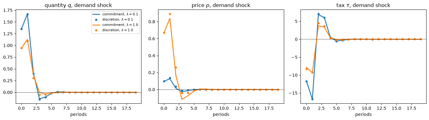
The iteration converges in a few steps.
Discretion produces higher losses than commitment, but only slightly: 0.2 percent higher with \(\lambda = 0.1\) and 0.7 percent with \(\lambda = 1\).
With \(\lambda = 0.1\) the paths are also close, even for the large taxes at dates 2 and 3 (7.07 against 6.88 at date 2); with \(\lambda = 1\) they differ more (4.48 against 3.76 at date 2), although the loss barely changes.
The small cost of discretion and the small gain from re-optimizing in Exercise 29.2 reflect the same fact: in this market, a policymaker gains little from promises about future taxes.
For the third part, we compute the date-0 policymaker’s best response directly.
The revisions that keep her successors’ rules satisfied form a line, a particular revision plus multiples of a null vector of the constraints, and the best response minimizes the loss along that line.
λ = 0.1
d_01, x_disc, _ = discretion(λ)
w = loss_weights(λ)
D_future = stack_rules(d_01)[1:]
A_c = D_future @ Θ_ν
ν_part, *_ = np.linalg.lstsq(A_c, -D_future @ x_A, rcond=None)
null = np.linalg.svd(A_c)[2][-1]
x_part, x_dir = x_A + Θ_ν @ ν_part, Θ_ν @ null
s_best = -np.sum(w * x_part * x_dir) / np.sum(w * x_dir**2)
best_response = x_part + s_best * x_dir
print(f"max |best response - discretionary path| = {np.abs(best_response - x_disc).max():.1e}")
max |best response - discretionary path| = 5.2e-14
Given that her successors follow \(\delta\), the date-0 policymaker’s best response is the discretionary path, so no policymaker wants to deviate.
Policy Counterfactuals in a New Keynesian Economy checks the same algorithm in a New Keynesian model, where it reproduces the familiar discretionary targeting rule.
Exercise 29.4
Use McKay and Wolf’s Proposition 1 to construct the “zeroing-out” counterfactual of Bernanke et al. [1997]: how would quantity and price respond to a supply shock if the government did not respond at all (\(\tilde\phi = 0\))?
Compare the McKay–Wolf answer with the truth and with the Sims–Zha answer.
Solution
x_A_s = M_inv_A @ forcing(0)
x_true_s = system_inverse(g_s, g_d, 0.0) @ forcing(0)
x_mw_s, _ = mw_counterfactual(M_inv_A, x_A_s, 0.0)
x_sz_s, _ = sims_zha(M_inv_A, x_A_s, 0.0)

fig, axes = plt.subplots(1, 3, figsize=(14, 4))
for i in range(3):
    axes[i].plot(split(x_A_s)[i][:H_plot], 'k:', lw=2, label=f"baseline, $\\phi = {φ_A}$")
    axes[i].plot(split(x_true_s)[i][:H_plot], 'C0', lw=2, label="true, no policy")
    axes[i].plot(split(x_mw_s)[i][:H_plot], 'C0o', ms=4, label="McKay–Wolf")
    axes[i].plot(split(x_sz_s)[i][:H_plot], 'C3--', lw=2, label="Sims–Zha")
    axes[i].axhline(0, color='k', lw=0.5)
    axes[i].set_title(f"{names[i]}, supply shock")
    axes[i].set_xlabel("periods")
axes[0].legend(fontsize=8)
plt.tight_layout()
plt.show()

print(f"max |McKay–Wolf - truth| = {np.abs(x_mw_s - x_true_s).max():.1e}")
print(f"max |Sims–Zha   - truth| = {np.abs(x_sz_s - x_true_s).max():.1e}")
for i, name in enumerate(["quantity", "price"]):
    effect = np.abs(split(x_true_s)[i] - split(x_A_s)[i]).max()
    error = np.abs(split(x_sz_s)[i] - split(x_true_s)[i]).max()
    print(f"{name}: peak response {np.abs(split(x_true_s)[i]).max():.4f}, largest policy effect "
          f"{effect:.4f}, Sims–Zha error / effect {error / effect:.2f}")
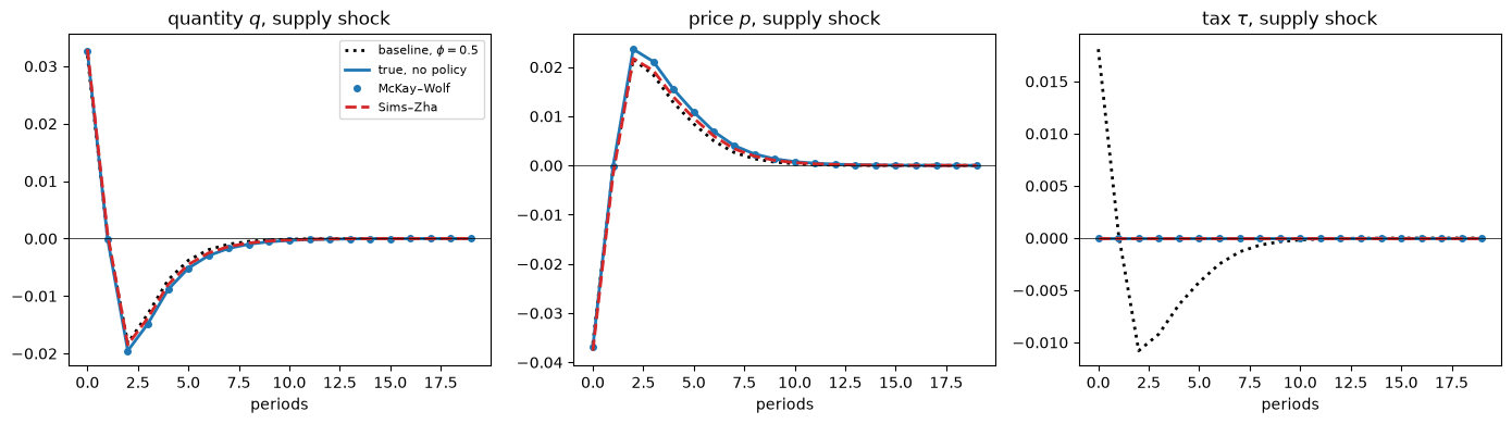
max |McKay–Wolf - truth| = 5.6e-17
max |Sims–Zha   - truth| = 1.9e-03
quantity: peak response 0.0326, largest policy effect 0.0017, Sims–Zha error / effect 0.61
price: peak response 0.0368, largest policy effect 0.0027, Sims–Zha error / effect 0.69
Again McKay and Wolf’s construction is exact, while the Sims–Zha construction, which keeps agents expecting the baseline rule, is not.
The policy effect is small here: removing the baseline rule changes the response of quantity by at most about 0.002, against a peak response of about 0.033.
The Sims–Zha error is about 60 percent as large as the effect itself for quantity and about 70 percent for the price.
Exercise 29.5
McKay and Wolf’s construction is exact when \(x_A(\varepsilon)\) and \(\Theta_\nu\) are known exactly.
Suppose instead that \(\Theta_\nu\) is measured with error, and recompute the counterfactual response to a demand shock under \(\tilde\phi = 2\) in 50 draws of the error.
Multiply each column of \(\Theta_\nu\) by an independent factor \(1 + 0.1\,\xi_\ell\), with \(\xi_\ell \sim N(0, 1)\), as if the size of each policy shock were mismeasured.
Instead, add to the quantity and price rows of each column a smooth error, an AR(1) path with autocorrelation 0.8 and standard deviation equal to 5 percent of that column’s peak response, leaving the tax rows unchanged.
Explain the difference.
Solution
rng_noise = np.random.default_rng(0)

def mw_from(Θ):
    "McKay–Wolf counterfactual under τ = -2 p from the baseline paths x_A and responses Θ."
    R_new = rule_block(φ_new)
    return x_A + Θ @ np.linalg.solve(R_new @ Θ, -R_new @ x_A)

def smooth_errors(Θ, ρ=0.8, size=0.05):
    "AR(1) errors in the quantity and price rows, scaled by each column's peak response."
    E = np.zeros_like(Θ)
    for b in range(2):
        z = rng_noise.standard_normal((T, Θ.shape[1]))
        e = np.zeros_like(z)
        for t in range(T):
            e[t] = ρ * e[t - 1] + np.sqrt(1 - ρ**2) * z[t] if t > 0 else z[0]   # stationary from t = 0
        E[b * T:(b + 1) * T] = size * e * np.abs(Θ[b * T:(b + 1) * T]).max(axis=0)
    return E

errors_scale = [cf_error(mw_from(Θ_ν * (1 + 0.1 * rng_noise.standard_normal(T))))
                for _ in range(50)]
errors_smooth = [cf_error(mw_from(Θ_ν + smooth_errors(Θ_ν))) for _ in range(50)]
print(f"mismeasured shock sizes: largest counterfactual error, q {np.max(errors_scale, axis=0)[0]:.1e}, "
      f"p {np.max(errors_scale, axis=0)[1]:.1e}")
print(f"smooth errors in (q, p): median counterfactual error, q {np.median(errors_smooth, axis=0)[0]:.3f}, "
      f"p {np.median(errors_smooth, axis=0)[1]:.3f}; 90th percentile, "
      f"q {np.percentile(errors_smooth, 90, axis=0)[0]:.3f}, p {np.percentile(errors_smooth, 90, axis=0)[1]:.3f}")
mismeasured shock sizes: largest counterfactual error, q 2.6e-16, p 4.6e-16
smooth errors in (q, p): median counterfactual error, q 0.047, p 0.017; 90th percentile, q 0.056, p 0.021
Mismeasuring the size of each policy shock does no harm at all: rescaling a column of \(\Theta_\nu\) rescales the shock that the construction chooses, and the counterfactual is unchanged.
What matters, as The baseline rule does not matter emphasizes, is the effect of each path of the tax on quantity and price.
Errors in those effects, of about 5 percent of each response’s peak, produce errors of about 5 percent in the counterfactual for quantity and 2 percent for the price.
The precision of McKay and Wolf’s counterfactual is the precision with which the effects of tax paths are measured.