
30. Policy Regimes and the Lucas Critique#
30.1. Overview#
Lucas [1976] proposed to evaluate a policy rule by computing outcomes in an economy whose private agents understand the rule and expect it to persist.
McKay and Wolf [2023] compute such outcomes from impulse responses to policy shocks; Policy Counterfactuals from Impulse Responses applies their method to a market for a single good.
They describe their thought experiment, in which a monetary policy rule links the interest rate \(i\) to inflation \(\pi\):
Note that this thought experiment supposes that the private sector perfectly understands the change in rule: the new relationship between \(i\) and \(\pi\) holds for all \(t \geq 0\).
Their counterfactual is a scenario: a rule announced at date 0, believed by everyone, and kept forever.
Sargent and Wallace [1976] questioned the internal consistency of that experiment:
… new rules are not adopted in a vacuum. Something would cause the change – a change in administrations, new appointments, and so on. Moreover, if rational agents live in a world in which rules can be and are changed, their behavior should take into account such possibilities and should depend on the process generating the rule changes.
Sims [1982] described most policy changes as realizations of a policy process that private agents already understand.
Sims and Zha [2006] linked vector autoregressions with regime-switching coefficients to the Lucas critique:
… once we recognize that changes in policy must in principle themselves be modeled as stochastic, Lucas’s argument can be seen as a claim that a certain sort of nonlinearity is important. Even if the public believes that policy is time-varying and tries to adjust its expectation formation accordingly, its behavior could be well approximated as linear and non-time-varying.
This lecture builds a model in which policy rules switch according to a Markov chain that private agents know.
The model is the market of Dynamic Supply and Demand Curves and Policy Counterfactuals from Impulse Responses, with a tax rule whose coefficient depends on the state of the chain.
The machinery is the Markov jump linear quadratic dynamic programming of Markov Jump Linear Quadratic Dynamic Programming.
The lecture
constructs a planning problem whose solution is the market equilibrium under switching policy regimes,
computes decision rules that depend on the current regime and on the probabilities of future regimes,
distinguishes a switch between regimes of a known process from a change in the process itself,
compares a permanent, credible rule with a reform that agents expect may be reversed,
tests McKay and Wolf’s construction when the historical rule switched regimes, and
fits vector autoregressions to data generated by switching regimes.
Three questions about policy rules call for three approaches.
question |
approach |
source of credibility |
|---|---|---|
what would happen if a rule were announced at date 0 and believed forever? |
scenario analysis, as in Policy Counterfactuals from Impulse Responses |
assumed |
which rules would a government choose and be able to sustain? |
dynamic programming squared, as in Sustainable Plans for a Calvo Model and Accounting for Monetary and Fiscal Policy |
the government’s incentives |
what happens when rule changes are realizations of a process that agents know? |
Markov-switching regimes, this lecture |
transition probabilities |
We use the following imports.
import numpy as np
import matplotlib.pyplot as plt
30.2. A market with policy regimes#
We use the parameters of Dynamic Supply and Demand Curves, except that we set the demander’s adjustment cost to zero, \(g_d = 0\).
With \(g_d = 0\) the market equilibrium under switching regimes solves a Markov jump linear quadratic planning problem.
The supplier chooses \(q_t\) to maximize
and the demander’s inverse demand curve is
The cost and demand shocks are \(s_t = B_s(L) w_{st}\) and \(d_t = B_d(L) w_{dt}\), as in Dynamic Supply and Demand Curves.
A Markov state \(s^p_t \in \{1, \ldots, m\}\) with transition matrix \(\Pi\) selects the policy regime.
The government sets the tax by the rule
where \(\phi_i\) is the feedback coefficient in regime \(i\) and \(\nu_t\) collects contemporaneous and news shocks to the rule, as in Policy Counterfactuals from Impulse Responses.
Private agents observe \(s^p_t\) and know \(\Pi\).
30.2.1. An equivalent planning problem#
Suppliers receive \(p_t - \tau_t = (1 + \phi_{s^p_t}) p_t - \nu_t\).
The supplier’s Euler equation and the demand curve imply
Equation (30.2) is the first-order condition of a planner who chooses \(\{q_t\}\) to minimize
The planner weights the area under the inverse demand curve at date \(t\) by \(1 + \phi_{s^p_t}\).
The weight enters only the date-\(t\) term because demand is static.
With \(g_d > 0\) the demander’s benefit at date \(t\) depends on \(q_t, \ldots, q_{t-4}\).
The first-order condition for \(q_t\) would then collect terms dated \(t, \ldots, t+4\), each weighted by the regime prevailing at its own date, and no single weight would apply.
With a single regime, dividing the objective by \(1 + \phi\) restates the result of Policy Counterfactuals from Impulse Responses: a price-stabilizing rule is equivalent to suppliers with cost parameters \(h_s/(1+\phi)\) and \(g_s/(1+\phi)\) and cost shocks \(s_t/(1+\phi)\).
The planner’s state vector is
where the last block is a queue of policy shocks that agents know at date \(t\).
The control is \(u_t = q_t\).
The one-period loss is \(x_t' R x_t + u_t' Q_i u_t + 2 u_t' N_i x_t\) in regime \(i\); only \(Q_i\) and \(N_i\) depend on the regime.
The matrix \(N_i\) is the matrix \(W_i\) of Markov Jump Linear Quadratic Dynamic Programming.
h_s = h_d = 1.0
g_s = 10.0
β = 1 / 1.05
B_d = np.convolve(np.convolve([1, .6], [1, .4]), [1, .2])
B_s = np.convolve(np.convolve([1, -.8], [1, .4]), [1, .2])
σ_s, σ_d = np.sqrt(0.5), 2.0

H = 60                               # length of the queue of policy shocks
n = 1 + 4 + 4 + H                    # dimension of the state
i_ws, i_wd, i_ν = 1, 5, 9            # positions of w_s,t, w_d,t, and ν_t

A = np.zeros((n, n))
A[2:5, 1:4] = np.eye(3)              # shift lagged cost shocks
A[6:9, 5:8] = np.eye(3)              # shift lagged demand shocks
A[i_ν:i_ν + H - 1, i_ν + 1:] = np.eye(H - 1)   # advance the queue of policy shocks
B = np.zeros((n, 1)); B[0, 0] = 1.0  # q_t becomes next period's q_{t-1}
C = np.zeros((n, 2)); C[i_ws, 0] = σ_s; C[i_wd, 1] = σ_d

e_q = np.zeros(n); e_q[0] = 1.0
s_sel = np.zeros(n); s_sel[1:5] = B_s
d_sel = np.zeros(n); d_sel[5:9] = B_d
ν_sel = np.zeros(n); ν_sel[i_ν] = 1.0

def loss_matrices(φ):
    "Q_i, R, N_i for the regime with feedback coefficient φ."
    ω = 1 + φ
    Q = np.array([[(h_s + g_s + ω * h_d) / 2]])
    R = g_s / 2 * np.outer(e_q, e_q)
    N = ((-g_s * e_q + s_sel + ν_sel + ω * d_sel) / 2).reshape(1, n)
    return Q, R, N
30.2.2. Linked Riccati equations#
The planner’s losses \(x' P_i x + \rho_i\) satisfy the linked Riccati equations of Markov Jump Linear Quadratic Dynamic Programming, with \(\bar P_i = \sum_j \Pi_{ij} P_j\):
The decision rule in regime \(i\) is \(q_t = -F_i x_t\) with \(F_i = (Q_i + \beta B' \bar P_i B)^{-1} (\beta B' \bar P_i A + N_i)\).
We code the iteration directly.
def solve_regimes(φs, Π, tol=1e-12, max_iter=20_000):
    "Decision rules F_i for regimes with feedback coefficients φs and transition matrix Π."
    m = len(φs)
    mats = [loss_matrices(φ) for φ in φs]
    P = np.zeros((m, n, n))
    for _ in range(max_iter):
        P_new = np.empty_like(P)
        for i, (Q, R, N) in enumerate(mats):
            P_bar = np.tensordot(Π[i], P, axes=1)
            G = β * B.T @ P_bar @ A + N
            P_new[i] = (R + β * A.T @ P_bar @ A
                        - G.T @ np.linalg.solve(Q + β * B.T @ P_bar @ B, G))
        converged = np.max(np.abs(P_new - P)) < tol
        P = P_new
        if converged:
            break
    F = np.empty((m, 1, n))
    for i, (Q, R, N) in enumerate(mats):
        P_bar = np.tensordot(Π[i], P, axes=1)
        F[i] = np.linalg.solve(Q + β * B.T @ P_bar @ B, β * B.T @ P_bar @ A + N)
    return F
Quantity, price, and the tax are linear functions of \(x_t\) in each regime: \(q_t = -F_{s^p_t} x_t\), \(p_t = -d_t - h_d q_t\), and \(\tau_t = -\phi_{s^p_t} p_t + \nu_t\).
We check that the computed decision rules satisfy the supplier’s Euler equation (30.2) along a simulated path.
The conditional expectation is \(\mathbb{E}_t q_{t+1} = -\sum_k \Pi_{s^p_t k} F_k (A - B F_{s^p_t}) x_t\).
def euler_residual(F, φs, Π, T_sim=300, seed=0):
    "Largest violation of the supplier's Euler equation along a simulated path."
    rng = np.random.default_rng(seed)
    m = len(φs)
    x, s, worst = np.zeros(n), 0, 0.0
    for t in range(T_sim):
        q = -(F[s] @ x).item()
        p = -d_sel @ x - h_d * q
        x_mean = (A - B @ F[s]) @ x
        Eq_next = sum(Π[s, k] * -(F[k] @ x_mean).item() for k in range(m))
        lhs = (1 + φs[s]) * p - x[i_ν]
        rhs = s_sel @ x + h_s * q + g_s * ((1 + β) * q - x[0] - β * Eq_next)
        worst = max(worst, abs(lhs - rhs))
        x = x_mean + C @ rng.standard_normal(2)
        s = rng.choice(m, p=Π[s])
    return worst

φs = np.array([0.0, 2.0])            # laissez-faire and price stabilization
Π = np.array([[0.95, 0.05],
              [0.05, 0.95]])
F = solve_regimes(φs, Π)
print(f"switching regimes: max Euler residual = {euler_residual(F, φs, Π):.1e}")
switching regimes: max Euler residual = 1.8e-14
The decision rules satisfy the Euler equation to machine precision.
Expected responses to a shock condition on the regime at the date of the shock.
Let \(M_t(j) = \mathbb{E}[x_t \mathbb{1}\{s^p_t = j\} \mid x_0, s^p_0]\).
These conditional means satisfy \(M_{t+1}(k) = \sum_j \Pi_{jk} (A - B F_j) M_t(j)\), and the expected outcomes are sums over \(j\) of linear functions of \(M_t(j)\).
one = np.array([[1.0]])              # transition matrix of a single regime

def expected_responses(F, φs, Π, x0, s0, T=40):
    "E[(q_t, p_t, τ_t) | x_0, s_0] for t = 0, ..., T-1."
    m = len(φs)
    M = [x0 * (j == s0) for j in range(m)]
    out = np.zeros((T, 3))
    for t in range(T):
        q_j = [-(F[j] @ M[j]).item() for j in range(m)]
        p_j = [-d_sel @ M[j] - h_d * q_j[j] for j in range(m)]
        ν_t = sum(M[j][i_ν] for j in range(m))
        out[t] = sum(q_j), sum(p_j), sum(-φs[j] * p_j[j] for j in range(m)) + ν_t
        M = [sum(Π[j, k] * (A - B @ F[j]) @ M[j] for j in range(m)) for k in range(m)]
    return out

x0_demand = C @ np.array([0.0, -1.0])     # a positive demand shock of one standard deviation
x0_supply = C @ np.array([-1.0, 0.0])     # a favorable supply shock of one standard deviation
T_plot = 20
names = ["quantity $q$", "price $p$"]
With a single regime, the planner’s solution coincides with the sequence-space solution that Policy Counterfactuals from Impulse Responses computes for the market with a tax.
We stack the supplier’s Euler equation, the static demand curve, and the rule \(\tau_t = -\phi p_t\) for \(t = 0, \ldots, 199\), as in that lecture, and compare the two solutions for three rules.
def sequence_space(φ, shock, T_seq=200):
    "Paths of (q, p, τ) after a favorable supply shock (0) or a positive demand shock (1)."
    Φ_s = np.zeros((T_seq, T_seq))
    for t in range(T_seq):
        Φ_s[t, t] = h_s + g_s * (1 + β)
        if t >= 1:
            Φ_s[t, t - 1] = -g_s
        if t + 1 < T_seq:
            Φ_s[t, t + 1] = -g_s * β
    I, O = np.eye(T_seq), np.zeros((T_seq, T_seq))
    M = np.block([[-Φ_s, I, -I],          # supply:  p - τ - Φ_s q = s
                  [h_d * I, I, O],        # demand:  p + h_d q = -d
                  [O, φ * I, I]])         # rule:    τ + φ p = 0
    s, d = np.zeros(T_seq), np.zeros(T_seq)
    if shock == 0:
        s[:4] = -σ_s * B_s
    else:
        d[:4] = -σ_d * B_d
    x = np.linalg.solve(M, np.concatenate([s, -d, np.zeros(T_seq)]))
    return np.column_stack([x[:T_seq], x[T_seq:2 * T_seq], x[2 * T_seq:]])

for φ in [0.0, 0.5, 2.0]:
    F_φ = solve_regimes([φ], one)
    gap = max(np.abs(expected_responses(F_φ, [φ], one, x0, 0, 40) - sequence_space(φ, k)[:40]).max()
              for k, x0 in [(0, x0_supply), (1, x0_demand)])
    print(f"φ = {φ}: max |planner - sequence space| = {gap:.1e}")
φ = 0.0: max |planner - sequence space| = 8.9e-16
φ = 0.5: max |planner - sequence space| = 8.9e-16
φ = 2.0: max |planner - sequence space| = 8.9e-16
The two methods agree to machine precision.
30.3. Regime-dependent decision rules#
Regime 1 is laissez-faire, \(\phi_1 = 0\); regime 2 stabilizes the price, \(\phi_2 = 2\).
Each regime persists with probability 0.95.
We compare the switching economy with two economies in which one rule holds forever.
F_lf = solve_regimes([0.0], one)     # laissez-faire forever
F_st = solve_regimes([2.0], one)     # stabilization forever

print("feedback of q_t on q_(t-1)")
print(f"  switching:  laissez-faire regime {-F[0, 0, 0]:.4f},  stabilization regime {-F[1, 0, 0]:.4f}")
print(f"  permanent:  laissez-faire        {-F_lf[0, 0, 0]:.4f},  stabilization        {-F_st[0, 0, 0]:.4f}")
feedback of q_t on q_(t-1)
  switching:  laissez-faire regime 0.6502,  stabilization regime 0.5477
  permanent:  laissez-faire        0.6537,  stabilization        0.5456
The decision rule in each regime differs from the rule under the corresponding permanent policy.
The feedback of \(q_t\) on \(q_{t-1}\) is 0.650 in the laissez-faire regime and 0.654 under permanent laissez-faire, and 0.548 in the stabilization regime and 0.546 under permanent stabilization.
Agents in each regime attach probability 0.05 to a switch next period, and their decisions respond.
fig, axes = plt.subplots(1, 2, figsize=(12, 4))
for s0, color, label in [(0, 'C0', "laissez-faire"), (1, 'C1', "stabilization")]:
    switching = expected_responses(F, φs, Π, x0_demand, s0, T_plot)
    F_perm = F_lf if s0 == 0 else F_st
    permanent = expected_responses(F_perm, [φs[s0]], one, x0_demand, 0, T_plot)
    for i, ax in enumerate(axes):
        ax.plot(switching[:, i], color=color, lw=2,
                label=f"{label} regime, switching")
        ax.plot(permanent[:, i], color=color, lw=2, ls='--',
                label=f"{label} forever")
for i, ax in enumerate(axes):
    ax.axhline(0, color='k', lw=0.5)
    ax.set_title(names[i])
    ax.set_xlabel("periods")
axes[0].legend(fontsize=8)
plt.tight_layout()
plt.show()
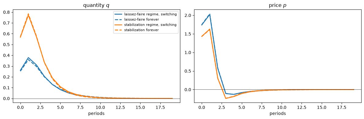
Fig. 30.1 Responses to a demand shock by regime#
On impact, a positive demand shock of one standard deviation raises quantity by 0.57 in the stabilization regime and by 0.26 in the laissez-faire regime.
The subsidy that holds down the price induces suppliers to produce more.
Under permanent rules the impact responses are 0.573 with stabilization and 0.252 with laissez-faire.
Each regime’s impact response lies between those two numbers, close to the response under the corresponding permanent rule.
The expected path averages over future switches, and decisions at each date anticipate them.
The impact response of quantity in each regime varies with the probability of a switch.
switch_probs = np.linspace(0, 0.5, 11)
impact = np.zeros((len(switch_probs), 2))
for k, pr in enumerate(switch_probs):
    Π_k = np.array([[1 - pr, pr], [pr, 1 - pr]])
    F_k = solve_regimes(φs, Π_k)
    for s0 in range(2):
        impact[k, s0] = expected_responses(F_k, φs, Π_k, x0_demand, s0, 1)[0, 0]

fig, ax = plt.subplots()
ax.plot(switch_probs, impact[:, 0], 'o-', lw=2, label="laissez-faire regime")
ax.plot(switch_probs, impact[:, 1], 's-', lw=2, label="stabilization regime")
ax.set_xlabel("probability of a switch next period")
ax.set_ylabel("impact response of $q$ to a demand shock")
ax.legend()
plt.show()
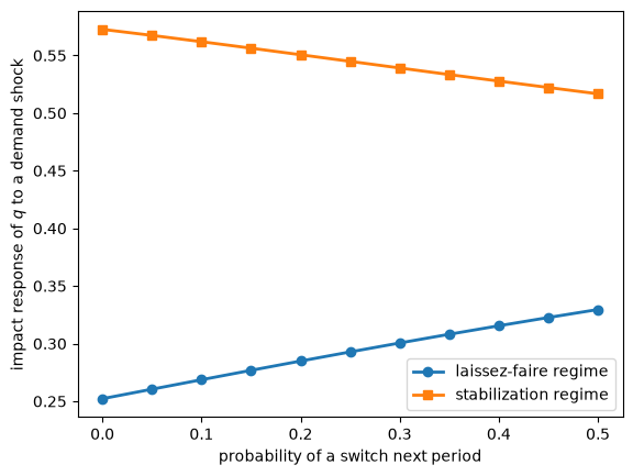
Fig. 30.2 Impact responses and switching probability#
As switches become more likely, the decision rules in the two regimes move toward each other.
With switching probability 0.5, the impact responses are 0.33 and 0.52; with permanent regimes, they are 0.25 and 0.57.
30.4. Two levels of the Lucas critique#
The switching economy distinguishes two kinds of policy change.
A switch from one regime to another of a known process leaves the decision rules \(F_1, F_2\) unchanged.
An econometrician who conditions on the regime can estimate those rules from history and use them to predict outcomes after a switch.
That is the setting that Sims [1982] regarded as typical of policy analysis.
A change in the process — the menu \(\{\phi_i\}\) or the transition matrix \(\Pi\) — changes the decision rules in every regime.
That is the setting of Lucas [1976].
A reform that may arrive illustrates the second kind of change.
The economy starts in the laissez-faire regime; each period a reform to the stabilization rule occurs with probability \(r\), and the reform is permanent.
print(" r      feedback on q_(t-1)   impact q   q one period later")
for r in [0.0, 0.05, 0.2]:
    Π_r = np.array([[1 - r, r], [0.0, 1.0]])
    F_r = solve_regimes(φs, Π_r)
    resp = expected_responses(F_r, φs, Π_r, x0_demand, 0, 2)
    print(f"{r:4.2f}   {-F_r[0, 0, 0]:20.4f}   {resp[0, 0]:8.4f}   {resp[1, 0]:17.4f}")
 r      feedback on q_(t-1)   impact q   q one period later
0.00                 0.6537     0.2522              0.3600
0.05                 0.6501     0.2604              0.3785
0.20                 0.6410     0.2847              0.4333
The prospect of a reform changes behavior under laissez-faire before any reform occurs.
With \(r = 0.2\) the feedback of \(q_t\) on \(q_{t-1}\) falls from 0.654 to 0.641, and the impact response of quantity to a demand shock rises from 0.252 to 0.285.
An econometrician who estimated the laissez-faire decision rule from a period in which no reform was in prospect would mispredict behavior once a reform became possible.
A change in the process can also change whether an equilibrium is unique.
Davig and Leeper [2007] show that, with Markov-switching interest-rate rules, the conditions for a unique bounded equilibrium depend on the whole switching process.
Our planning problem has a strictly convex objective, and every rule and every switching process in this lecture delivers a unique equilibrium.
30.5. Scenarios and regime changes#
McKay and Wolf’s counterfactual is the stabilization rule announced at date 0 and kept forever.
In a regime-switching economy, a reform to the stabilization rule may be reversed.
We let the stabilization regime end with probability \(e\) each period and compute the expected response to a demand shock that occurs just after a reform.
fig, ax = plt.subplots()
for e, ls in [(0.0, '-'), (0.05, '--'), (0.2, '-.'), (0.5, ':')]:
    Π_e = np.array([[0.95, 0.05], [e, 1 - e]])
    F_e = solve_regimes(φs, Π_e)
    resp = expected_responses(F_e, φs, Π_e, x0_demand, 1, T_plot)
    label = "permanent reform" if e == 0 else f"exit probability {e}"
    ax.plot(resp[:, 0], lw=2, ls=ls, color='C1', label=label)
ax.axhline(0, color='k', lw=0.5)
ax.set_xlabel("periods")
ax.set_ylabel("expected response of $q$")
ax.legend()
plt.show()
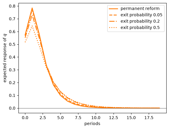
Fig. 30.3 Reversible and permanent reforms#
On impact and in the two periods that follow, the more likely a reversal, the smaller the response of quantity.
With exit probability 0.2, the response of quantity one period after the shock is about 7 percent smaller than under a permanent reform; with exit probability 0.5, it is about 18 percent smaller.
Two forces produce the gap.
Agents who expect a reversal adjust less to the reformed rule; the expected path also averages over reversals that occur.
From the fourth period after the shock on, the response under every reversible reform exceeds the response under the permanent reform, because a reversal returns the economy to laissez-faire, under which quantity adjusts more slowly.
McKay and Wolf’s scenario corresponds to \(e = 0\).
The dynamic programming squared lectures, such as Sustainable Plans for a Calvo Model and Accounting for Monetary and Fiscal Policy, study what determines the credibility that this lecture summarizes by \(e\).
30.6. McKay and Wolf in a regime-switching economy#
Suppose that the historical data come from the switching economy.
An econometrician estimates expected responses to the demand shock and to contemporaneous and news shocks to the tax rule, conditional on the regime at the date of the shock.
McKay and Wolf’s construction from Policy Counterfactuals from Impulse Responses uses these expected responses.
The supplier’s Euler equation and the demand curve are linear with coefficients that do not depend on the regime.
By the law of iterated expectations, expected paths of \((q, p, \tau)\) satisfy those equations.
A counterfactual rule \(\tau_t = -\tilde \phi p_t\) that holds forever is a linear restriction on expected paths.
McKay and Wolf’s construction recovers the permanent counterfactual exactly.
T_mw = 40

def stacked(resp):
    return np.concatenate([resp[:, 0], resp[:, 1], resp[:, 2]])

def mw_from_switching(F, φs, Π, s0, φ_new):
    "McKay–Wolf counterfactual from expected responses in the switching economy."
    x_A = stacked(expected_responses(F, φs, Π, x0_demand, s0, T_mw))
    Θ = np.column_stack([stacked(expected_responses(F, φs, Π, np.eye(n)[i_ν + ℓ], s0, T_mw))
                         for ℓ in range(T_mw)])
    R_new = np.hstack([np.zeros((T_mw, T_mw)), φ_new * np.eye(T_mw), np.eye(T_mw)])
    ν = np.linalg.solve(R_new @ Θ, -R_new @ x_A)
    return (x_A + Θ @ ν).reshape(3, T_mw).T, x_A.reshape(3, T_mw).T

truth = expected_responses(F_st, [2.0], one, x0_demand, 0, T_mw)
for s0, label in [(0, "laissez-faire"), (1, "stabilization")]:
    cf, x_A = mw_from_switching(F, φs, Π, s0, 2.0)
    print(f"data from the {label} regime: baseline impact on q {x_A[0, 0]:.4f}, "
          f"max |McKay–Wolf - permanent stabilization| = {np.abs(cf[:30] - truth[:30]).max():.1e}")
data from the laissez-faire regime: baseline impact on q 0.2604, max |McKay–Wolf - permanent stabilization| = 3.4e-14
data from the stabilization regime: baseline impact on q 0.5674, max |McKay–Wolf - permanent stabilization| = 3.8e-14
The baseline responses depend on the regime at the date of the shock.
From either regime, the construction recovers the response under a permanent stabilization rule to machine precision.
A switching historical rule does not impair McKay and Wolf’s construction.
The construction does not deliver the reversible reform of the previous section.
Under a rule that may revert, the expected tax is \(\mathbb{E}_0 \tau_t = -\sum_j \phi_j \mathbb{E}_0 [p_t \mathbb{1}\{s^p_t = j\}] + \mathbb{E}_0 \nu_t\).
That restriction involves the joint distribution of prices and regimes and is not a linear restriction on expected paths.
Computing it requires a model of the regime process.
30.7. Vector autoregressions fit to regime-switching data#
Because the switching economy is covariance stationary, \(\{(q_t, p_t)\}\) has an infinite-order vector autoregression with constant coefficients: the population linear least-squares projection of \((q_t, p_t)\) on its entire past.
Its coefficients differ from those of the law of motion of \(x_t\), because \((q_t, p_t)\) is not a Markov process.
Two reasons apply even with a single rule: the shocks are moving averages, and under either of our two rules the supply shock is not fundamental for \((q_t, p_t)\), as Exercise 30.3 verifies.
With switching regimes, the history of \((q_t, p_t)\) also carries information about the regime.
The innovations of the vector autoregression are serially uncorrelated but conditionally heteroskedastic.
We simulate long samples from the switching economy and from the two economies in which one rule holds forever.
The simulations set the policy shocks \(\nu_t\) to zero.
The econometrician fits autoregressions of orders 1, 4, and 8 to \((q_t, p_t)\) and ignores the tax rate, which would reveal the regime.
def simulate(F, φs, Π, T_sim, seed):
    "Simulate (q_t, p_t) and the regime."
    rng = np.random.default_rng(seed)
    m = len(φs)
    A_F = [A - B @ F[j] for j in range(m)]
    qp = np.zeros((T_sim, 2))
    regime = np.zeros(T_sim, dtype=int)
    x, s = np.zeros(n), 0
    for t in range(T_sim):
        q = -(F[s] @ x).item()
        qp[t] = q, -d_sel @ x - h_d * q
        regime[t] = s
        x = A_F[s] @ x + C @ rng.standard_normal(2)
        s = rng.choice(m, p=Π[s])
    return qp, regime

def var_fit(y, lags):
    "Least-squares autoregression of y_t on y_(t-1), ..., y_(t-lags): coefficients and residuals."
    Y = y[lags:]
    X = np.hstack([y[lags - k:len(y) - k] for k in range(1, lags + 1)])
    coef, *_ = np.linalg.lstsq(X, Y, rcond=None)
    return coef, Y - X @ coef

T_sim = 200_000
qp, regime = simulate(F, φs, Π, T_sim, seed=1234)
qp_lf, _ = simulate(F_lf, [0.0], one, T_sim, seed=1234)
qp_st, _ = simulate(F_st, [2.0], one, T_sim, seed=1234)

print("residual variance of q")
print("lags   switching   laissez-faire forever   stabilization forever")
for lags in [1, 4, 8]:
    v = [var_fit(y, lags)[1][:, 0].var() for y in (qp, qp_lf, qp_st)]
    print(f"{lags:4d}   {v[0]:9.4f}   {v[1]:21.4f}   {v[2]:21.4f}")

_, U = var_fit(qp, 8)
reg = regime[8:]
print(f"\nswitching economy, order 8: residual variance of q in the laissez-faire regime "
      f"{U[reg == 0, 0].var():.4f}, in the stabilization regime {U[reg == 1, 0].var():.4f}")
residual variance of q
lags   switching   laissez-faire forever   stabilization forever
   1      0.2512                  0.0779                  0.3991
   4      0.2016                  0.0657                  0.3300
   8      0.2013                  0.0653                  0.3293

switching economy, order 8: residual variance of q in the laissez-faire regime 0.0741, in the stabilization regime 0.3273
From order 1 to order 8, the residual variance of quantity falls by 20 percent in the switching economy, 16 percent under permanent laissez-faire, and 17 percent under permanent stabilization.
Most of the gain reflects the moving-average shocks, which are present with a single rule.
In the switching economy, the residual variance of quantity is more than four times larger in the stabilization regime than in the laissez-faire regime.
Within the laissez-faire regime, the residual variance of the pooled autoregression, 0.074, exceeds the residual variance of an autoregression fit to data from an economy that stays in laissez-faire forever, 0.065.
To separate the sources of that gap, we use the tax rate to classify the sample by regime.
We keep observations whose eight lags lie in the same regime as the current observation, and fit a separate autoregression of order 8 within each regime.
lags = 8
Y = qp[lags:]
X = np.hstack([qp[lags - k:len(qp) - k] for k in range(1, lags + 1)])
same = np.array([np.all(regime[t - lags:t + 1] == regime[t]) for t in range(lags, T_sim)])
U_pooled = var_fit(qp, lags)[1]
for j, label in [(0, "laissez-faire"), (1, "stabilization")]:
    keep = same & (reg == j)
    coef_j, *_ = np.linalg.lstsq(X[keep], Y[keep], rcond=None)
    U_j = Y[keep] - X[keep] @ coef_j
    print(f"{label:14s}: residual variance of q, regime-specific {U_j[:, 0].var():.4f}, "
          f"pooled {U_pooled[keep, 0].var():.4f}")
laissez-faire : residual variance of q, regime-specific 0.0699, pooled 0.0718
stabilization : residual variance of q, regime-specific 0.3232, pooled 0.3249
In the laissez-faire regime, dropping observations whose lags straddle a switch lowers the pooled residual variance from 0.074 to 0.072.
Fitting separate coefficients lowers it further to 0.070.
The remaining gap to 0.065 reflects a laissez-faire decision rule that anticipates switches.
In both regimes, conditioning on the regime lowers the residual variance of quantity by less than 3 percent.
The autoregression’s innovation in the price, orthogonalized by ordering the price first, is mostly a demand shock.
On impact, a demand shock of one standard deviation moves the price by 1.74 in the laissez-faire regime and by 1.43 in the stabilization regime; a supply shock of one standard deviation moves it by 0.03.
We compare the response of quantity to that innovation with the responses of quantity to a demand shock in each regime, each scaled to raise the price by one unit on impact.
lags = 8
coef, U = var_fit(qp, lags)
B_var = [coef[2 * k:2 * k + 2].T for k in range(lags)]      # y_t = Σ_k B_k y_(t-k) + u_t
Ψ = [np.eye(2)]
for h in range(1, T_plot):
    Ψ.append(sum(B_var[k] @ Ψ[h - 1 - k] for k in range(min(lags, h))))
swap = np.array([[0, 1], [1, 0]])
L_p = swap @ np.linalg.cholesky(swap @ np.cov(U.T) @ swap) @ swap
var_resp = np.array([Ψ_h @ L_p[:, 1] for Ψ_h in Ψ])         # price ordered first
var_resp /= var_resp[0, 1]

fig, ax = plt.subplots()
for s0, color, label in [(0, 'C0', "laissez-faire regime"), (1, 'C1', "stabilization regime")]:
    resp = expected_responses(F, φs, Π, x0_demand, s0, T_plot)
    ax.plot(resp[:, 0] / resp[0, 1], color=color, lw=2, label=label)
ax.plot(var_resp[:, 0], 'k--', lw=2, label="autoregression, price innovation")
ax.axhline(0, color='k', lw=0.5)
ax.set_xlabel("periods")
ax.set_ylabel("response of $q$ per unit impact on $p$")
ax.legend()
plt.show()
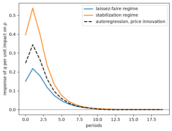
Fig. 30.4 Autoregression and regime responses#
On impact, the autoregression’s response is 0.25 per unit of price, against 0.15 in the laissez-faire regime and 0.40 in the stabilization regime.
A constant-coefficient autoregression averages over regimes.
In the passage quoted in the overview, Sims and Zha [2006] conjecture that such an approximation can describe behavior well.
In our market, the constant-coefficient autoregression fits almost as well as autoregressions that condition on the regime, and its impulse response describes behavior in neither regime.
Hamilton [1989] showed how to estimate a model whose coefficients switch with an unobserved Markov state.
30.8. Summary#
We constructed a Markov equilibrium model of market for a good in which policy rules switch according to a Markov chain that agents know, and computed it by solving a Markov jump linear quadratic planning problem.
Decision rules depend on the current regime and on the probabilities of future regimes.
A switch within a known process leaves decision rules unchanged; a change in the process changes them in every regime.
A reform that agents expect may be reversed has smaller effects in the first periods after a shock than the same reform made permanent and credible.
McKay and Wolf’s construction recovers outcomes under a permanent rule from data generated by switching regimes; it does not deliver outcomes under a rule that may be reversed.
A constant-coefficient vector autoregression fit to regime-switching data averages over regimes and has conditionally heteroskedastic innovations; it fits almost as well as autoregressions that condition on the regime, and its impulse responses describe behavior in neither regime.
30.9. Exercises#
Exercise 30.1
McKay and Wolf’s construction above uses expected responses conditional on the regime at the date of the shock.
Suppose instead that the econometrician averages the expected responses over the stationary distribution of the regime.
Show that the construction still recovers the response under a permanent stabilization rule, and explain why.
Solution
The stationary distribution of the symmetric chain is \((0.5, 0.5)\).
def averaged(x0, weights):
    return sum(w * stacked(expected_responses(F, φs, Π, x0, s0, T_mw))
               for s0, w in enumerate(weights))

weights = [0.5, 0.5]
x_A = averaged(x0_demand, weights)
Θ = np.column_stack([averaged(np.eye(n)[i_ν + ℓ], weights) for ℓ in range(T_mw)])
R_new = np.hstack([np.zeros((T_mw, T_mw)), 2.0 * np.eye(T_mw), np.eye(T_mw)])
ν = np.linalg.solve(R_new @ Θ, -R_new @ x_A)
cf = (x_A + Θ @ ν).reshape(3, T_mw).T
print(f"max |McKay–Wolf - permanent stabilization| = {np.abs(cf[:30] - truth[:30]).max():.1e}")
max |McKay–Wolf - permanent stabilization| = 3.6e-14
Each conditional expected path satisfies the linear Euler equation and demand curve, and so does any weighted average of them.
The construction needs only that the baseline paths and the responses to policy shocks satisfy the private sector’s equations, and that the counterfactual rule is a linear restriction on paths.
Exercise 30.2
Two regime processes can have the same stationary distribution and different persistence.
Compare the symmetric chain with switching probability 0.05 to a symmetric chain with switching probability 0.25.
Compute the expected response of quantity to a demand shock in each regime under each chain, and explain the differences.
Solution
fig, axes = plt.subplots(1, 2, figsize=(12, 4))
for pr, ls in [(0.05, '-'), (0.25, '--')]:
    Π_k = np.array([[1 - pr, pr], [pr, 1 - pr]])
    F_k = solve_regimes(φs, Π_k)
    for s0, ax in enumerate(axes):
        resp = expected_responses(F_k, φs, Π_k, x0_demand, s0, T_plot)
        ax.plot(resp[:, 0], lw=2, ls=ls, label=f"switching probability {pr}")
for ax, title in zip(axes, ["laissez-faire regime", "stabilization regime"]):
    ax.axhline(0, color='k', lw=0.5)
    ax.set_title(title)
    ax.set_xlabel("periods")
axes[0].legend()
plt.tight_layout()
plt.show()
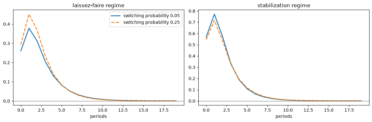
With more frequent switches, agents in each regime expect the other regime sooner.
Responses in the laissez-faire regime rise toward those in the stabilization regime, and responses in the stabilization regime fall toward those in the laissez-faire regime.
The expected paths also average over more switches along the path.
The stationary distribution alone does not determine behavior; persistence of the regimes matters.
Exercise 30.3
In Policy Counterfactuals from Impulse Responses, a sufficiently aggressive price-stabilizing rule makes the supply shock fundamental for \((q_t, p_t)\).
Repeat that calculation for the static-demand market of this lecture.
For permanent rules \(\phi \in \{0, 2, 4, 6, 8, 10\}\), compute the moving-average representation of \((q_t, p_t)\) in terms of the two structural shocks, the innovation covariance \(V\) of its Wold representation, and \(\|L^{-1} d_s\|\), where \(L\) is the Cholesky factor of \(V\) and \(d_s\) is the impact response to the supply shock.
For an economy that switches between \(\phi = 0\) and \(\phi = 8\), say in which regime a rotation of the innovations of a vector autoregression for \((q_t, p_t)\) could recover the supply shock, and explain why the answer is approximate.
Hint: write the moving-average representation, truncated after 80 lags, in state-space form and solve the Kalman filter’s Riccati equation with scipy.linalg.solve_discrete_are.
Solution
The structural moving-average coefficients are the expected responses to the two shocks.
The steady-state Kalman filter for the truncated moving average delivers the innovation covariance \(V\), as in Dynamic Supply and Demand Curves.
from scipy.linalg import solve_discrete_are

H_ma = 80

def ma_coefficients(φ):
    "D_j (2 x 2): responses of (q, p) at lag j to the supply and demand shocks under a permanent rule φ."
    F_φ = solve_regimes([φ], one)
    D = np.zeros((H_ma, 2, 2))
    for k, x0 in enumerate([x0_supply, x0_demand]):
        D[:, :, k] = expected_responses(F_φ, [φ], one, x0, 0, H_ma)[:, :2]
    return D

def innovation_covariance(D):
    "Innovation covariance of the Wold representation of z_t = Σ_j D_j ε_(t-j)."
    k = D.shape[2]
    A_ma = np.zeros((H_ma * k, H_ma * k)); A_ma[k:, :-k] = np.eye((H_ma - 1) * k)
    C_ma = np.zeros((H_ma * k, k)); C_ma[:k] = np.eye(k)
    G = np.hstack(list(D))
    R_meas = 1e-10 * np.eye(2)
    Σ = solve_discrete_are(A_ma.T, G.T, C_ma @ C_ma.T, R_meas, balanced=False)
    return G @ Σ @ G.T + R_meas

print(" φ    ||L^-1 d_s||   ||L^-1 d_d||")
for φ in [0.0, 2.0, 4.0, 6.0, 8.0, 10.0]:
    D = ma_coefficients(φ)
    L = np.linalg.cholesky(innovation_covariance(D))
    norms = np.linalg.norm(np.linalg.solve(L, D[0]), axis=0)
    print(f"{φ:4.1f}   {norms[0]:12.4f}   {norms[1]:12.4f}")
 φ    ||L^-1 d_s||   ||L^-1 d_d||
 0.0         0.8090         1.0000
 2.0         0.8992         1.0000
 4.0         0.9527         1.0000
 6.0         0.9899         1.0000
 8.0         1.0000         1.0000
10.0         1.0000         1.0000
The demand shock is fundamental under every rule.
The supply shock is not fundamental under laissez-faire; it becomes fundamental between \(\phi = 6\) and \(\phi = 8\), a more aggressive rule than the market with dynamic demand of Policy Counterfactuals from Impulse Responses requires.
An economy that switches between \(\phi = 0\) and \(\phi = 8\) alternates between a regime in which a vector autoregression for \((q_t, p_t)\) cannot recover the supply shock and a regime in which a rotation of its innovations can.
The statement is approximate, because regime-conditional decision rules differ from those under permanent rules; it becomes exact as the regimes become permanent.
A constant-coefficient autoregression fit to the pooled data mixes the two regimes.