70. Gradualism in Self-Enforcing Trade Agreements#
70.1. Overview#
Free-trade agreements rarely eliminate tariffs at once.
The North American Free Trade Agreement phased out tariffs between the United States and Mexico over 15 years, the United Kingdom’s accession to the European Community eliminated internal tariffs over five years, and GATT negotiations lowered tariffs round by round.
If governments could commit to tariffs and if goods and factor markets worked well, immediate free trade would be efficient [Mussa, 1986].
Governments cannot commit, so trade agreements must be self-enforcing: each government must prefer to honor the agreement, given that a deviation would trigger a trade war.
This lecture studies two papers that use this requirement to explain gradualism.
Bond and Park [2002] show that when two countries differ in size, the efficient self-enforcing agreement can start with a positive tariff and move toward free trade, even though the economic environment never changes.
Bond [2009] shows that self-enforcement can make it efficient to add members to an agreement one at a time.
Bond and Park compute the frontier of self-enforcing agreements recursively, with the payoff promised to one country as the state variable.
That makes their problem one of dynamic programming squared: the value function of the problem appears inside its own constraints, as in Credible Government Policies in a Model of Chang, International Lending with Moral Hazard and Risk of Repudiation, and Capital Flows Under Moral Hazard.
The key force is backloading: an agreement relaxes the incentive constraint of the country tempted to deviate by promising it more in the future, and a tariff imposed by its partner, which the tempted country cannot escape by deviating, serves as a transfer in the meantime.
The next lecture, Institution Building Without Commitment, studies gradual liberalization with a different equilibrium concept, one that does not rely on the threat of a permanent trade war.
We use the following imports.
import numpy as np
import matplotlib.pyplot as plt
from collections import namedtuple
from scipy.optimize import minimize_scalar
70.2. A two-country trade model#
There are two goods and two countries, a small country \(S\) and a large country \(L\).
In country \(S\), demand and supply of good \(i\) are
and in country \(L\) they are \(\lambda\) times as large,
where \(\lambda \ge 1\) measures the relative size of \(L\).
Following Bond and Park [2002], we set \(\alpha_1^L = \alpha_2^S > \alpha_2^L = \alpha_1^S\), so that \(S\) imports good 1 and exports good 2, and the countries are mirror images when \(\lambda = 1\).
Each country taxes its imports with a specific tariff: \(t_S\) on good 1 imported by \(S\), and \(t_L\) on good 2 imported by \(L\).
Domestic prices satisfy \(p_1^S = p_1^L + t_S\) and \(p_2^L = p_2^S + t_L\), and world market clearing for each good gives
National welfare \(W_j(t_j, t_k)\) is the sum of consumer surplus, producer surplus, and tariff revenue over the two goods.
Bond and Park [2002] show that
\(W_j\) is concave in the country’s own tariff and is maximized at
\[ t_L^N = \frac{\lambda (\alpha_2^S - \alpha_2^L)}{(1 + 2\lambda)(\beta + B)} , \qquad t_S^N = \frac{\alpha_1^L - \alpha_1^S}{(2 + \lambda)(\beta + B)} ; \]\(W_j\) is decreasing and convex in the other country’s tariff;
world welfare \(W_S + W_L\) is maximized at free trade.
Because the welfare of each country is additively separable in the two tariffs, \(t_j^N\) is a dominant strategy, and the pair \((t_S^N, t_L^N)\) is the Nash equilibrium of the one-shot tariff game.
The game is a prisoner’s dilemma: each country gains by taxing imports, which improves its terms of trade, but both would be better off at free trade, at least when they are not too different in size.
The large country’s Nash tariff rises with \(\lambda\), and the small country’s falls toward zero, because a small country cannot move world prices.
TradeModel = namedtuple('TradeModel', ('A', 'B', 'β', 'α_hi', 'α_lo', 'λ', 'δ'))

def create_trade_model(A=100.0, B=1.0, β=1.0, α_hi=-40.0, α_lo=-60.0, λ=1.1, δ=0.8):
    "α_hi = α_1^L = α_2^S and α_lo = α_2^L = α_1^S."
    return TradeModel(A=A, B=B, β=β, α_hi=α_hi, α_lo=α_lo, λ=λ, δ=δ)

def welfare(t_S, t_L, m):
    "National welfare (W_S, W_L) when S taxes good 1 at t_S and L taxes good 2 at t_L."
    A, B, β, α_hi, α_lo, λ = m.A, m.B, m.β, m.α_hi, m.α_lo, m.λ
    p_1L = ((1 + λ) * A - α_lo - λ * α_hi - (B + β) * t_S) / ((1 + λ) * (B + β))
    p_2S = ((1 + λ) * A - α_hi - λ * α_lo - λ * (B + β) * t_L) / ((1 + λ) * (B + β))
    p_1S, p_2L = p_1L + t_S, p_2S + t_L
    CS = lambda p: (A - B * p)**2 / (2 * B)               # consumer surplus
    PS = lambda p, α: (α + β * p)**2 / (2 * β)            # producer surplus
    imports = lambda p, α: (A - B * p) - (α + β * p)
    W_S = (CS(p_1S) + PS(p_1S, α_lo) + CS(p_2S) + PS(p_2S, α_hi)
           + t_S * imports(p_1S, α_lo))
    W_L = λ * (CS(p_1L) + PS(p_1L, α_hi) + CS(p_2L) + PS(p_2L, α_lo)
               + t_L * imports(p_2L, α_lo))
    return W_S, W_L

def nash_tariffs(m):
    A, B, β, α_hi, α_lo, λ = m.A, m.B, m.β, m.α_hi, m.α_lo, m.λ
    t_LN = λ * (α_hi - α_lo) / ((1 + 2 * λ) * (β + B))
    t_SN = (α_hi - α_lo) / ((2 + λ) * (β + B))
    return t_SN, t_LN
We check the formulas for the Nash tariffs by maximizing each country’s welfare numerically.
m = create_trade_model()
t_SN, t_LN = nash_tariffs(m)
best_S = minimize_scalar(lambda t: -welfare(t, 0, m)[0], bounds=(0, 20), method='bounded').x
best_L = minimize_scalar(lambda t: -welfare(0, t, m)[1], bounds=(0, 20), method='bounded').x
print(f"Nash tariffs: t_S = {t_SN:.3f} (numerical {best_S:.3f}),  t_L = {t_LN:.3f} "
      f"(numerical {best_L:.3f})")
print("welfare at free trade:", np.round(welfare(0, 0, m), 1),
      "  at the Nash tariffs:", np.round(welfare(t_SN, t_LN, m), 1))
Nash tariffs: t_S = 3.226 (numerical 3.226),  t_L = 3.438 (numerical 3.438)
welfare at free trade: [1354.9 1479.9]   at the Nash tariffs: [1347.3 1475.8]
70.3. Self-enforcing agreements#
A trade agreement is a sequence of tariffs \(t_j(i) \ge 0\) and side payments \(s_j(i) \ge 0\) that country \(j\) pays at date \(i = 0, 1, \ldots\).
Side payments stand for concessions in side agreements, such as rules on intellectual property or foreign investment.
The payoff to country \(j\) from date \(i\) on is
If governments could commit, efficient agreements would eliminate tariffs immediately and use side payments to divide the gains, so the first-best frontier is
Without commitment, an agreement must be self-enforcing.
Following Bond and Park [2002], we assume that a deviation triggers permanent reversion to the Nash tariffs without side payments, which gives country \(j\) the payoff \(V_j^N = W_j(t_j^N, t_k^N) / (1 - \delta)\).
A deviating country sets its Nash tariff and stops paying side payments, but it still receives the side payment of its partner in the period of deviation.
The incentive constraint of country \(j\) at each date \(i\) is therefore
70.3.1. Stationary free-trade agreements#
Consider free trade with constant side payments.
The incentive constraint (70.1) becomes \(s_j - \delta s_k \le H_j\), where
weighs the future loss from a trade war against the one-period gain from deviating.
Since only one country pays in an efficient agreement, the largest net side payment that country \(j\) is willing to make each period is \(T_j = H_j\) if \(H_j > 0\) and \(T_j = H_j / \delta\) if \(H_j \le 0\), in which case \(j\) must be paid at least \(-T_j\).
A free-trade agreement with constant side payments is sustainable if and only if \(T_S + T_L \ge 0\), and then it can give \(L\) any payoff in the interval \([V_L^*, V_L^{**}]\), where
Below \(V_L^*\), the large country gets too little to stay in a free-trade agreement; above \(V_L^{**}\), the small country does.
def stationary_bounds(m):
    "Nash payoffs, maximal side payments, and the interval [V_L*, V_L**] of sustainable free trade."
    δ = m.δ
    t_SN, t_LN = nash_tariffs(m)
    W_S0, W_L0 = welfare(0, 0, m)
    W_SN, W_LN = welfare(t_SN, t_LN, m)
    H_S = δ * (W_S0 - W_SN) - (1 - δ) * (welfare(t_SN, 0, m)[0] - W_S0)
    H_L = δ * (W_L0 - W_LN) - (1 - δ) * (welfare(0, t_LN, m)[1] - W_L0)
    T_S = H_S if H_S > 0 else H_S / δ
    T_L = H_L if H_L > 0 else H_L / δ
    return dict(V_SN=W_SN / (1 - δ), V_LN=W_LN / (1 - δ), T_S=T_S, T_L=T_L,
                V_L_low=(W_L0 - T_L) / (1 - δ), V_L_high=(W_L0 + T_S) / (1 - δ))

models = {"λ = 1.1, δ = 0.8": create_trade_model(λ=1.1, δ=0.8),
          "λ = 1.5, δ = 0.7": create_trade_model(λ=1.5, δ=0.7)}
for name, m_i in models.items():
    sb = stationary_bounds(m_i)
    print(f"{name}: T_S = {sb['T_S']:.2f}, T_L = {sb['T_L']:.2f};  "
          f"V_L* - V_L^N = {sb['V_L_low'] - sb['V_LN']:.2f}, "
          f"V_L** - V_L^N = {sb['V_L_high'] - sb['V_LN']:.2f}")
λ = 1.1, δ = 0.8: T_S = 4.45, T_L = 1.37;  V_L* - V_L^N = 13.50, V_L** - V_L^N = 42.58
λ = 1.5, δ = 0.7: T_S = 8.50, T_L = -7.53;  V_L* - V_L^N = 19.29, V_L** - V_L^N = 22.51
We study two cases.[1]
When \(\lambda = 1.1\) and \(\delta = 0.8\), both \(T_S\) and \(T_L\) are positive: each country would pay something to keep free trade.
When \(\lambda = 1.5\) and \(\delta = 0.7\), \(T_L < 0\), so the small country must pay for access to the large country’s market; the large country also wins the tariff war, in the sense that it does better at the Nash equilibrium than at free trade.
70.4. A recursive formulation#
Outside \([V_L^*, V_L^{**}]\), stationary free-trade agreements are not self-enforcing.
To find the efficient agreements there, Bond and Park [2002] treat the payoff promised to the large country as a state variable.
Let \(\tilde \Omega(V_L)\) be the largest payoff that the small country can get from a self-enforcing agreement that gives the large country \(V_L\).
It satisfies
subject to
where \(y\) is the payoff promised to \(L\) from next period on.
The first constraint delivers the promised payoff to \(L\), and the other two are the incentive constraints (70.1) of \(L\) and \(S\).
The unknown function \(\tilde \Omega\) appears in the objective and in the small country’s incentive constraint, which is what makes this dynamic programming squared.
When the promise-keeping constraint binds, the net side payment is \(s_S - s_L = V_L - W_L - \delta y\), and the objective becomes
world welfare today plus the discounted world value of the continuation, minus what is promised to \(L\).
Bond and Park [2002] show that \(\tilde \Omega\) is the limit of the sequence obtained by applying the right side of (70.2) repeatedly to the first-best frontier, building on Rustichini [1998].
They also show that a country never imposes a tariff while making a side payment, and their characterization implies that at most one country imposes a tariff at a time, so we search over one tariff at a time.
def solve_frontier(m, n_V=601, n_t=161, tol=1e-9, max_iter=100):
    """
    Iterate on the Bellman equation for the incentive-constrained frontier, starting
    from the first-best frontier, on a grid of promised payoffs to L.
    """
    δ = m.δ
    t_SN, t_LN = nash_tariffs(m)
    sb = stationary_bounds(m)
    W_S0, W_L0 = welfare(0, 0, m)
    V_L_max = welfare(0, t_LN, m)[1] - W_L0 + sb['V_L_high']    # see the text
    V = np.unique(np.r_[np.linspace(sb['V_LN'], V_L_max, n_V), sb['V_L_low'], sb['V_L_high']])
    # among equally good continuations, prefer free trade in [V_L*, V_L**]
    tie_break = 1e-7 * ((V >= sb['V_L_low']) & (V <= sb['V_L_high']))

    # candidate tariff pairs: one tariff at a time
    t_grid = np.linspace(0, 1, n_t)
    t_S = np.r_[np.zeros(n_t), t_SN * t_grid[1:]]
    t_L = np.r_[t_LN * t_grid, np.zeros(n_t - 1)]
    W_S, W_L = welfare(t_S, t_L, m)
    gain_L = welfare(0, t_L, m)[1] - welfare(0, t_LN, m)[1]     # W_L(t_L, ·) - W_L(t_L^N, ·)
    gain_S = welfare(t_S, 0, m)[0] - welfare(t_SN, 0, m)[0]

    Ω = (W_S0 + W_L0) / (1 - δ) - V                             # first-best frontier
    for it in range(max_iter):
        Ω_new = np.empty_like(Ω)
        best = np.empty((len(V), 2), dtype=int)
        for j, v in enumerate(V):
            net = v - W_L[:, None] - δ * V[None, :]              # s_S - s_L, promise kept
            s_S, s_L = np.maximum(net, 0), np.maximum(-net, 0)
            feasible = ((gain_L[:, None] - s_L + δ * V[None, :] >= δ * sb['V_LN'] - 1e-9)
                        & (gain_S[:, None] - s_S + δ * Ω[None, :] >= δ * sb['V_SN'] - 1e-9))
            obj = np.where(feasible, (W_S + W_L)[:, None] - v + δ * (V + Ω)[None, :], -np.inf)
            k = np.argmax(obj + tie_break[None, :])
            best[j] = np.unravel_index(k, obj.shape)
            Ω_new[j] = obj[tuple(best[j])]
        # L may also be given more than promised: take the best over payoffs V' >= V
        source = np.empty(len(V), dtype=int)
        source[-1] = len(V) - 1
        for j in range(len(V) - 2, -1, -1):
            source[j] = j if Ω_new[j] >= Ω_new[source[j + 1]] else source[j + 1]
        Ω_new = Ω_new[source]
        change = np.max(np.abs(Ω_new - Ω))
        Ω = Ω_new
        if change < tol:
            break
    i_t, i_y = best[source, 0], best[source, 1]
    return dict(V=V, Ω=Ω, t_S=t_S[i_t], t_L=t_L[i_t], y=V[i_y], iterations=it + 1, **sb)

solutions = {name: solve_frontier(m_i) for name, m_i in models.items()}
for name, sol in solutions.items():
    print(f"{name}: converged after {sol['iterations']} iterations")
λ = 1.1, δ = 0.8: converged after 2 iterations
λ = 1.5, δ = 0.7: converged after 2 iterations
The iteration converges after one application of the Bellman operator, followed by a check that a second application changes nothing.
The reason is the main result of Bond and Park [2002]: the continuation \(y\) always lies where first-best payoffs are attainable, so the continuation value is the first-best one.
Several continuations are then equally good, and the code picks one in \([V_L^*, V_L^{**}]\), where free trade with constant side payments is self-enforcing.
For payoffs above \(V_L^{**}\), where only the small country’s incentive constraint binds, Bond and Park [2002] also give the frontier in closed form, which we use to check the computation.
Along it, the small country’s incentive constraint binds, so \(\tilde \Omega = W_S(t_S^N, t_L) + \delta V_S^N\), and the large country gets \(V_L = W_L(t_L, 0) - W_L(0, 0) + V_L^{**}\), for \(t_L \in [0, t_L^N]\); the largest payoff to \(L\), used to set the grid above, is the one with \(t_L = t_L^N\).
for name, m_i in models.items():
    sol = solutions[name]
    t_SN, t_LN = nash_tariffs(m_i)
    t_check = np.linspace(0, t_LN, 9)
    V_L = welfare(0, t_check, m_i)[1] - welfare(0, 0, m_i)[1] + sol['V_L_high']
    Ω_closed = welfare(t_SN, t_check, m_i)[0] + m_i.δ * sol['V_SN']
    gap = np.abs(np.interp(V_L, sol['V'], sol['Ω']) - Ω_closed).max()
    print(f"{name}: max |computed - closed form| above V_L** = {gap:.3f}")
λ = 1.1, δ = 0.8: max |computed - closed form| above V_L** = 0.056
λ = 1.5, δ = 0.7: max |computed - closed form| above V_L** = 0.070
The small differences come from the grids of tariffs and promised payoffs.
fig, axes = plt.subplots(2, 2, figsize=(12, 8))
for col, (name, sol) in enumerate(solutions.items()):
    V, Ω = sol['V'], sol['Ω']
    W0 = sum(welfare(0, 0, models[name]))
    ax = axes[0, col]
    ax.plot(V - sol['V_LN'], W0 / (1 - models[name].δ) - V - sol['V_SN'], 'k--', lw=1,
            label="first best")
    ax.plot(V - sol['V_LN'], Ω - sol['V_SN'], 'C0', lw=2, label="self-enforcing")
    ax.set_title(name)
    ax.set_xlabel(r"$V_L - V_L^N$")
    ax.set_ylabel(r"$V_S - V_S^N$")
    ax = axes[1, col]
    ax.plot(V - sol['V_LN'], sol['t_S'], 'C1', lw=2, label=r"first-period $t_S$")
    ax.plot(V - sol['V_LN'], sol['t_L'], 'C2', lw=2, label=r"first-period $t_L$")
    ax.set_xlabel(r"$V_L - V_L^N$")
    ax.set_ylabel("tariff")
    for a in axes[:, col]:
        for x in [sol['V_L_low'], sol['V_L_high']]:
            a.axvline(x - sol['V_LN'], color='gray', ls=':', lw=1)
axes[0, 0].legend()
axes[1, 0].legend()
plt.tight_layout()
plt.show()
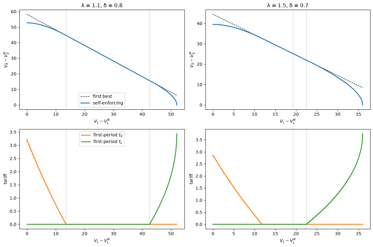
Fig. 70.1 Frontiers of trade agreements#
The top panels show the two frontiers, measured from the Nash payoffs; the dotted lines mark \(V_L^*\) and \(V_L^{**}\).
Between them, free trade with constant side payments is self-enforcing and the two frontiers coincide.
Above \(V_L^{**}\), the small country is asked to pay so much that it would rather deviate.
The efficient agreement then lets the large country tax its imports in the first period: the small country can stop a side payment by deviating, but it cannot escape a tariff.
From the second period on, the agreement switches to free trade with a payoff to \(L\) in \([V_L^*, V_L^{**}]\), so the tariff falls in two steps, from \(t_L^N\) to a first-period tariff and then to zero.
Below \(V_L^*\), the same logic applies with the roles reversed, and the small country imposes the first-period tariff.
When \(T_L < 0\) (right panels), there is a range below \(V_L^*\) in which first-best payoffs can still be reached without tariffs, by lowering the small country’s first-period side payment.
The constrained frontier is strictly below the first-best frontier wherever a tariff is used, and in every case the payoff of the constrained country rises over time: the agreement promises it more later in exchange for less now.
70.5. Consumption smoothing and many-step liberalization#
In the model so far, liberalization takes only two steps.
Bond and Park [2002] show that it becomes gradual when the small country wants to smooth its consumption, for example because it lacks access to international capital markets.
Let \(S\) be infinitesimally small, so that it cannot affect world prices, its Nash tariff is zero, and \(t_S = 0\) in any efficient agreement.
Prices in \(S\) are then \(p_1^S = p_1^{LA}\) and \(p_2^S = p_2^{LA} - t_L\), where \(p_i^{LA} = (A - \alpha_i^L)/(B + \beta)\) are the large country’s autarky prices.
The large country’s welfare from the agreement is its tariff revenue, \(W_L(t_L) = t_L \big[ X_2^S(p_2^S) - D_2^S(p_2^S) \big]\), which is maximized at \(t_L^N = (\alpha_2^S - \alpha_2^L) / \big(2 (B + \beta)\big)\).
The small country’s payoff in a period is \(U\big(W_S(t_L) + s_L - s_S\big)\), with \(U\) strictly concave, while the large country’s payoff stays linear.
70.5.1. Where the large country’s incentive constraint binds#
With free trade, the large country’s payoff is the side payment it receives, and its incentive constraint requires that it receive at least \(W_L(t_L^N) / \delta\) per period, so stationary free trade is self-enforcing only for \(V_L \ge V_L^* = V_L^N / \delta\), where \(V_L^N = W_L(t_L^N) / (1 - \delta)\).
Bond and Park [2002] show that for \(V_L \in (V_L^N, V_L^*)\) the large country’s incentive constraint binds, the small country’s does not, and the small country pays a side payment, so \(s_L = 0\).
The binding incentive constraint of \(L\) and the promise-keeping constraint then pin down
so that the only choice left is the tariff, and the Bellman equation becomes
where \(\tilde \Omega(y) = U\big(W_S(0) - (1 - \delta) y\big) / (1 - \delta)\) on the first-best region \(y \in [V_L^*, V_L^{**}]\).
Because \(W_L(t_L) \ge 0\), the continuation \(y\) never exceeds \(V_L^*\), and it reaches \(V_L^*\) only when \(t_L = 0\).
A tariff \(t_L > 0\) lowers the payoff \(y\) promised to \(L\) for the future, so it slows the rise in the small country’s side payment.
The agreement trades a static distortion, the tariff, against an intertemporal one, an uneven consumption path for \(S\), and it reduces both gradually.
We use the demand and supply parameters of the previous section, \(\delta = 0.9\), and constant relative risk aversion, \(U(c) = \left[ (c/\bar c)^{1 - \gamma} - 1 \right] / (1 - \gamma)\), with consumption scaled by its free-trade level \(\bar c = W_S(0)\).
The side payments are small relative to the small country’s surplus, less than 4 percent of it, so the consumption-smoothing motive matters only when curvature is high, and we show results for \(\gamma \in \{5, 20, 50\}\).
We start each agreement at \(V_L = V_L^N\), the point on the frontier that gives the small country all the gains, and check that the small country’s incentive constraint is slack along the solution, as Proposition 3 of Bond and Park [2002] asserts.
SmallCountry = namedtuple('SmallCountry', ('A', 'B', 'β', 'α_hi', 'α_lo', 'δ', 'γ'))

def create_small_country(A=100.0, B=1.0, β=1.0, α_hi=-40.0, α_lo=-60.0, δ=0.9, γ=20.0):
    return SmallCountry(A=A, B=B, β=β, α_hi=α_hi, α_lo=α_lo, δ=δ, γ=γ)

def small_country_welfare(t_L, sc):
    "The small country's surplus W_S(t_L) and the large country's tariff revenue W_L(t_L)."
    A, B, β, α_hi, α_lo = sc.A, sc.B, sc.β, sc.α_hi, sc.α_lo
    p_1 = (A - α_hi) / (B + β)                   # L's autarky price of good 1
    p_2 = (A - α_lo) / (B + β) - t_L             # price of good 2 in S
    W_S = ((A - B * p_1)**2 / (2 * B) + (α_lo + β * p_1)**2 / (2 * β)
           + (A - B * p_2)**2 / (2 * B) + (α_hi + β * p_2)**2 / (2 * β))
    W_L = t_L * ((α_hi + β * p_2) - (A - B * p_2))
    return W_S, W_L

def solve_smoothing(sc, n_V=600, n_t=600, tol=1e-13, max_iter=5000):
    "Iterate on the Bellman equation where L's incentive constraint binds."
    δ, γ = sc.δ, sc.γ
    t_N = (sc.α_hi - sc.α_lo) / (2 * (sc.B + sc.β))
    W_S0 = small_country_welfare(0.0, sc)[0]
    if γ == 1:
        U = lambda c: np.log(c / W_S0)
    else:
        U = lambda c: ((c / W_S0)**(1 - γ) - 1) / (1 - γ)
    V_N = small_country_welfare(t_N, sc)[1] / (1 - δ)
    V_low = V_N / δ
    Ω_first_best = lambda y: U(W_S0 - (1 - δ) * y) / (1 - δ)

    V = np.linspace(V_N, V_low, n_V)
    t = np.linspace(0, t_N, n_t)
    W_S, W_L = small_country_welfare(t, sc)
    y = (V_N - W_L) / δ                           # L's binding incentive constraint
    Ω = Ω_first_best(V)
    for it in range(max_iter):
        Ωy = np.where(y >= V_low, Ω_first_best(y), np.interp(y, V, Ω))
        obj = U(W_S[None, :] - (V[:, None] - V_N)) + δ * Ωy[None, :]
        Ω_new = obj.max(axis=1)
        if np.max(np.abs(Ω_new - Ω)) < tol:
            Ω = Ω_new
            break
        Ω = Ω_new

    def policy(v):
        "The optimal tariff at promised payoff v, by continuous maximization."
        def rhs(tt):
            W_S_t, W_L_t = small_country_welfare(tt, sc)
            yy = (V_N - W_L_t) / δ
            Ωy = Ω_first_best(yy) if yy >= V_low else np.interp(yy, V, Ω)
            return U(W_S_t - (v - V_N)) + δ * Ωy
        return minimize_scalar(lambda tt: -rhs(tt), bounds=(0, t_N), method='bounded',
                               options={'xatol': 1e-10}).x

    # slack in the small country's incentive constraint along the grid solution
    k = obj.argmax(axis=1)
    Ωy_k = np.where(y[k] >= V_low, Ω_first_best(y[k]), np.interp(y[k], V, Ω))
    V_SN = U(small_country_welfare(t_N, sc)[0]) / (1 - δ)
    ics_slack = (U(W_S[k] - (V - V_N)) + δ * Ωy_k) - (U(W_S[k]) + δ * V_SN)

    return dict(V=V, Ω=Ω, policy=policy, V_N=V_N, V_low=V_low, t_N=t_N, iterations=it + 1,
                min_ics_slack=ics_slack.min())

def simulate_agreement(sc, sol, n=30):
    "Tariffs, side payments, and promised payoffs, starting from V_L = V_L^N."
    v, path = sol['V_N'], []
    for i in range(n):
        if v >= sol['V_low']:                     # free trade from here on
            path.append((0.0, v - sol['V_N'], v))
            continue
        t_L = sol['policy'](v)
        path.append((t_L, v - sol['V_N'], v))
        v = (sol['V_N'] - small_country_welfare(t_L, sc)[1]) / sc.δ
    return np.array(path)

γ_values = [5, 20, 50]
paths = {}
for γ in γ_values:
    sc = create_small_country(γ=γ)
    sol = solve_smoothing(sc)
    paths[γ] = simulate_agreement(sc, sol)
    print(f"γ = {γ}: converged after {sol['iterations']} iterations;  smallest slack in S's "
          f"incentive constraint {sol['min_ics_slack']:.3f};  first tariffs {np.round(paths[γ][:5, 0], 3)}")
γ = 5: converged after 7 iterations;  smallest slack in S's incentive constraint 0.105;  first tariffs [0.829 0.259 0.087 0.029 0.009]
γ = 20: converged after 15 iterations;  smallest slack in S's incentive constraint 0.230;  first tariffs [1.497 0.759 0.415 0.235 0.135]
γ = 50: converged after 32 iterations;  smallest slack in S's incentive constraint 0.991;  first tariffs [1.942 1.189 0.783 0.537 0.376]
sc = create_small_country()
sol_ref = solve_smoothing(sc)
W_S_free = small_country_welfare(0.0, sc)[0]
fig, axes = plt.subplots(1, 3, figsize=(14, 4))
for γ in γ_values:
    t_L, s_S = paths[γ][:, 0], paths[γ][:, 1]
    consumption = small_country_welfare(t_L, sc)[0] - s_S
    axes[0].plot(t_L, 'o-', ms=3, lw=2, label=rf"$\gamma = {γ}$")
    axes[1].plot(s_S, 'o-', ms=3, lw=2)
    axes[2].plot(100 * (consumption / W_S_free - 1), 'o-', ms=3, lw=2)
axes[1].axhline(sol_ref['V_low'] - sol_ref['V_N'], color='gray', ls=':', lw=1)
for ax, title in zip(axes, ["large country's tariff $t_L$",
                            r"side payment $s_S = V_L - V_L^N$",
                            "small country's consumption (% from free trade)"]):
    ax.set_title(title)
    ax.set_xlabel("period")
axes[0].legend()
plt.tight_layout()
plt.show()
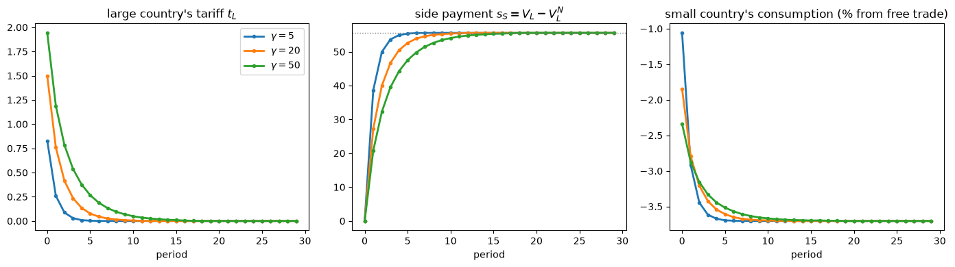
Fig. 70.2 Gradual liberalization with consumption smoothing#
The agreement starts with a positive tariff by the large country that declines period by period toward zero.
The side payment from the small country, which equals \(V_L - V_L^N\), rises toward \(V_L^* - V_L^N\), the dotted line, so the payoff promised to the large country rises toward the region where free trade is self-enforcing.
The small country’s consumption, its surplus net of the side payment, falls gradually rather than all at once.
The more the small country cares about smoothing its consumption, the higher the first tariff and the slower the liberalization.
Without curvature, the large country would be compensated entirely by a side payment that jumps after the first period, and no tariff would be used in this region; curvature makes a jump in side payments costly, so the agreement uses a declining tariff to slow their rise.
70.6. Gradual expansion of membership#
Bond [2009] asks a related question about who belongs to an agreement: when is it efficient to form a bilateral agreement first and to add a third country later?
There are three countries and three states: no agreement \(N\), a bilateral agreement \(B\) between countries 1 and 2, and a global agreement \(G\).
A country gets the flow payoff \(w(N)\), \(w(G)\), or, under \(B\), \(w_m(B)\) as a member and \(w_n(B)\) as the non-member, and it pays a one-time adjustment cost \(k\) when it joins an agreement, for example the cost of reallocating workers and of adapting its laws.
70.6.1. Commitment#
If countries could commit to agreements and side payments, an efficient path would maximize world welfare, the sum of the countries’ payoffs net of adjustment costs.
Let \(w^W(a)\) be the sum of the countries’ flow payoffs in state \(a\), so that \(w^W(G) = 3 w(G)\) and \(w^W(B) = 2 w_m(B) + w_n(B)\), and let \(C(a', a)\) be the sum of their adjustment costs of moving from \(a\) to \(a'\).
Starting from \(N\), forming \(B\) at date 0 and \(G\) at date 1 beats forming \(G\) at once if the adjustment costs it saves exceed the world welfare it forgoes for one period:
Bond [2009] assumes that a permanent move to \(G\) beats staying in any other state \(a\) forever, \(w^W(G) - (1 - \delta) C(G, a) > w^W(a)\).
When each country pays the same cost \(k\) whenever it joins an agreement, the left side of the inequality above is \((1 - \delta) k\), and the assumption for \(a = B\) says that \((1 - \delta) k < w^W(G) - w^W(B)\), so forming \(G\) at once maximizes world welfare.
Efficient delay with commitment needs adjustment costs that depend more strongly on the sequence of agreements, for example when adding a country costs less once a bilateral agreement is in place.
70.6.2. Self-enforcement#
Without commitment, each member of an agreement must prefer to honor it.
A member that deviates from an agreement \(a\) gets \(w^D(a)\) for one period, avoids the adjustment cost of joining, keeps any side payment it was supposed to pay, still receives any side payment owed to it, and then gets a punishment payoff \(w^P(a)\) forever.
The enforcement power of an agreement for a member, \(\Phi(a, \delta)\), is the excess of the member’s average payoff from the agreement over its average payoff from deviating, before side payments and adjustment costs: \(\Phi(G, \delta) = w(G) - \left[ (1 - \delta) w^D(G) + \delta w^P(G) \right]\), and \(\Phi(B, \delta)\) is defined in the same way with the member’s flow payoff \(w_m(B)\).
Bond [2009] shows that side payments should be backloaded: a side payment received at the date a country joins does not relax its incentive constraint, because it would receive it even if it deviated, so compensation should come in later periods.
A country \(i\) that joins with adjustment cost \(c_i\) can then be asked to pay at most
per period from the next period on, and the agreement is self-enforcing if and only if the maximal payments add up to a nonnegative number.
In an immediate global agreement, every country pays \(k\), so the agreement is self-enforcing if and only if \(\Phi(G, \delta) \ge (1 - \delta) k\).
A two-step agreement forms \(B\) at date 0 and adds country 3 at date 1.
At date 1, countries 1 and 2 are already members, so each can pay up to \(\Phi(G, \delta)\) per period from date 2 on to subsidize the newcomer, whose maximal payment is \(\left[ \Phi(G, \delta) - (1 - \delta) k \right] / \delta\).
The second step is therefore self-enforcing if and only if \((1 + 2\delta) \Phi(G, \delta) \ge (1 - \delta) k\).[2]
The smallest subsidy that each original member must then pay is \(s = \max\left\{0, \left[ (1 - \delta) k - \Phi(G, \delta) \right] / (2\delta) \right\}\), so from date 1 on an original member gets the average payoff \(w(G) - \delta s\).
At date 0, each of countries 1 and 2 pays \(k\) and gets \(w_m(B)\), so its incentive constraint is
The original members can subsidize the newcomer out of the slack enforcement power of the global agreement, which makes the second step easier to sustain than an immediate global agreement.
They must also be willing to stay in the first step, which is easier when the bilateral agreement has more enforcement power than the global one.
We compute the smallest discount factors that sustain each path for an example in which the bilateral agreement has more enforcement power, \(\Phi(B, \delta) = \Phi(G, \delta) + 1\), because a member of the bilateral agreement gains less by deviating and is punished more harshly.
Membership = namedtuple('Membership', ('w_G', 'w_D_G', 'w_P_G', 'w_mB', 'w_nB', 'w_D_B', 'w_P_B', 'k'))

def create_membership(w_G=12.0, w_D_G=14.0, w_P_G=10.0, w_mB=12.0, w_nB=9.5,
                      w_D_B=13.0, w_P_B=9.0, k=4.0):
    return Membership(w_G=w_G, w_D_G=w_D_G, w_P_G=w_P_G, w_mB=w_mB, w_nB=w_nB,
                      w_D_B=w_D_B, w_P_B=w_P_B, k=k)

def immediate_slack(δ, mb):
    Φ_G = mb.w_G - ((1 - δ) * mb.w_D_G + δ * mb.w_P_G)
    return Φ_G - (1 - δ) * mb.k

def two_step_slack(δ, mb):
    "The smaller of the slacks in the second-step and first-step constraints."
    Φ_G = mb.w_G - ((1 - δ) * mb.w_D_G + δ * mb.w_P_G)
    Φ_B = mb.w_mB - ((1 - δ) * mb.w_D_B + δ * mb.w_P_B)
    second = (1 + 2 * δ) * Φ_G - (1 - δ) * mb.k
    s = max(0.0, ((1 - δ) * mb.k - Φ_G) / (2 * δ))     # subsidy per original member
    first = Φ_B - (1 - δ) * mb.k + δ * (mb.w_G - δ * s - mb.w_mB)
    return min(second, first, Φ_G)

def min_discount_factor(slack, mb):
    "The smallest δ on a fine grid at which the slack is nonnegative."
    grid = np.linspace(0.01, 0.999, 9_000)
    ok = np.array([slack(δ, mb) >= 0 for δ in grid])
    return grid[ok.argmax()] if ok.any() else np.nan

mb = create_membership()
print(f"smallest δ: immediate global agreement {min_discount_factor(immediate_slack, mb):.3f}, "
      f"two-step agreement {min_discount_factor(two_step_slack, mb):.3f}")
δ = 0.7
print(f"at δ = {δ}: average world welfare of the two-step path minus the immediate path = "
      f"{(1 - δ) * ((1 - δ) * mb.k - (3 * mb.w_G - 2 * mb.w_mB - mb.w_nB)):.3f}")
smallest δ: immediate global agreement 0.750, two-step agreement 0.656
at δ = 0.7: average world welfare of the two-step path minus the immediate path = -0.390
In this example, the global agreement can be reached in two steps for discount factors at which an immediate global agreement would not be self-enforcing, even though, with commitment, the immediate path would yield higher world welfare.
The bilateral agreement is a building bloc: for discount factors between the two thresholds, without it the global agreement would never be reached.
The advantage comes from the bilateral agreement’s extra enforcement power: Exercise 70.3 shows that with the same enforcement power as the global agreement, the two-step path would need the same discount factor as the immediate one.
Bond [2009] shows more generally that whether the two-step path maximizes world welfare is neither necessary nor sufficient for it to be easier to sustain, because sustainability depends on deviation payoffs as well as on world welfare.
70.7. Connections to other lectures#
Institution Building Without Commitment also explains gradual trade liberalization, but with an equilibrium concept that does not rely on the threat of a permanent trade war; here, as in the best plans sustained by Markov reversion in that lecture, a single deviation ends cooperation forever.
Sustainable Plans for a Calvo Model and Credible Government Policies in a Model of Chang study sustainable plans; Bond and Park [2002] note that replacing Nash reversion with the harshest credible punishments of Abreu [1988] would enlarge the set of self-enforcing agreements without changing their shape over time.
International Lending with Moral Hazard and Risk of Repudiation and Capital Flows Under Moral Hazard study lending with moral hazard and a risk of repudiation, in which a value function enters the enforcement constraint; the backloading of payments to the party whose incentive constraint binds is the force that Thomas and Worrall [1994] found in contracts with a host country that cannot commit not to expropriate.
Repeated Moral Hazard and Optimal Unemployment Insurance use promised utility as the state variable in problems with hidden actions instead of limited commitment.
70.8. Exercises#
Exercise 70.1
The relative size \(\lambda\) of the large country determines who pays whom in a self-enforcing free-trade agreement.
Holding \(\delta = 0.8\) and the other parameters fixed, compute \(T_S\), \(T_L\), and the large country’s gain from the tariff war, \(W_L(t_L^N, t_S^N) - W_L(0, 0)\), for \(\lambda\) between 1 and 2.
For which \(\lambda\) does the large country win the tariff war?
For which \(\lambda\) can a free-trade agreement have the large country pay the small one?
Solution
λ_grid = np.linspace(1, 2, 101)
T_S, T_L, war_gain = [], [], []
for λ_i in λ_grid:
    m_i = create_trade_model(λ=λ_i, δ=0.8)
    sb = stationary_bounds(m_i)
    T_S.append(sb['T_S'])
    T_L.append(sb['T_L'])
    war_gain.append(welfare(*nash_tariffs(m_i), m_i)[1] - welfare(0, 0, m_i)[1])
T_S, T_L, war_gain = map(np.array, (T_S, T_L, war_gain))

fig, ax = plt.subplots()
ax.plot(λ_grid, T_S, lw=2, label=r"$T_S$")
ax.plot(λ_grid, T_L, lw=2, label=r"$T_L$")
ax.plot(λ_grid, war_gain, lw=2, label=r"$W_L^N - W_L(0, 0)$")
ax.axhline(0, color='k', lw=0.8)
ax.set_xlabel(r"relative size $\lambda$")
ax.legend()
plt.show()

print(f"L wins the tariff war for λ above {λ_grid[np.argmax(war_gain > 0)]:.2f}")
print(f"T_L > 0 for λ below {λ_grid[np.argmax(T_L < 0)]:.2f}")
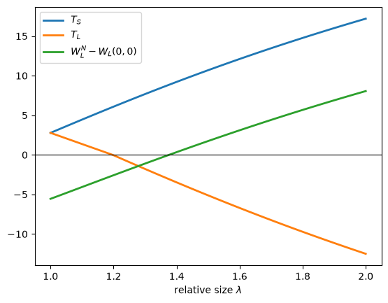
L wins the tariff war for λ above 1.38
T_L > 0 for λ below 1.20
The large country wins the tariff war once it is about 38 percent larger than the small country, and from then on any free-trade agreement must have the small country pay for access.
The large country is willing to pay for free trade only when the countries are close in size, for \(\lambda\) below about 1.2 when \(\delta = 0.8\); a larger \(\lambda\) raises its gain from deviating relative to the cost of the trade war.
At \(\delta = 0.8\), the small country is willing to pay throughout this range, and more so the larger its partner.
Exercise 70.2
In Consumption smoothing and many-step liberalization, compute the number of periods it takes for the large country’s tariff to fall below one percent of its first-period value, for \(\gamma \in \{5, 20, 50\}\) and \(\delta \in \{0.85, 0.9, 0.95\}\).
How do the speed of liberalization and the first-period tariff depend on \(\gamma\) and \(\delta\)?
Solution
print("   δ    γ    first tariff   periods to fall below 1% of it")
for δ_i in [0.85, 0.9, 0.95]:
    for γ in [5, 20, 50]:
        sc = create_small_country(δ=δ_i, γ=γ)
        path = simulate_agreement(sc, solve_smoothing(sc), n=200)
        t_path = path[:, 0]
        n_below = np.argmax(t_path < 0.01 * t_path[0])
        print(f"{δ_i:5.2f} {γ:4d}   {t_path[0]:11.3f}   {n_below:12d}")
   δ    γ    first tariff   periods to fall below 1% of it
 0.85    5         0.866              5
 0.85   20         1.552              9
 0.85   50         2.011             15
 0.90    5         0.829              5
 0.90   20         1.497              9
 0.90   50         1.942             13
 0.95    5         0.798              5
 0.95   20         1.444              8
 0.95   50         1.875             12
More curvature raises the first-period tariff and slows liberalization, because smoothing the small country’s consumption matters more.
A higher discount factor lowers the first-period tariff and slightly speeds liberalization.
Exercise 70.3
In Gradual expansion of membership, vary the adjustment cost \(k\) from 0 to 8 and compute
the smallest discount factors that sustain the immediate and the two-step paths, and
at \(\delta = 0.8\), whether the two-step path would yield higher world welfare under commitment.
Find values of \(k\) at which the two-step path is easier to sustain even though it yields lower world welfare, and repeat the calculation with \(w^D(B) = 14\) and \(w^P(B) = 10\), which give the bilateral agreement the same enforcement power as the global one.
Solution
def step_slacks(δ, mb):
    "Slacks in the second-step and first-step constraints of the two-step path."
    Φ_G = mb.w_G - ((1 - δ) * mb.w_D_G + δ * mb.w_P_G)
    Φ_B = mb.w_mB - ((1 - δ) * mb.w_D_B + δ * mb.w_P_B)
    s = max(0.0, ((1 - δ) * mb.k - Φ_G) / (2 * δ))
    return (1 + 2 * δ) * Φ_G - (1 - δ) * mb.k, Φ_B - (1 - δ) * mb.k + δ * (mb.w_G - δ * s - mb.w_mB)

δ = 0.8
print("   k   smallest δ: immediate  two-step  (binding step)   same enforcement power"
      "   two-step better with commitment")
for k in [0, 1, 2, 4, 6, 8]:
    mb_k = create_membership(k=k)
    mb_same = create_membership(k=k, w_D_B=14.0, w_P_B=10.0)
    δ_two = min_discount_factor(two_step_slack, mb_k)
    second, first = step_slacks(δ_two, mb_k)
    binding = "first" if first < second else "second"
    better = (1 - δ) * k > 3 * mb_k.w_G - 2 * mb_k.w_mB - mb_k.w_nB
    print(f"{k:4.0f}   {min_discount_factor(immediate_slack, mb_k):19.3f}  {δ_two:8.3f}"
          f"  {'(' + binding + ')':<8s}       {min_discount_factor(two_step_slack, mb_same):18.3f}"
          f"   {str(better):>14s}")
   k   smallest δ: immediate  two-step  (binding step)   same enforcement power   two-step better with commitment
   0                 0.500     0.500  (second)                    0.500            False
   1                 0.600     0.553  (second)                    0.600            False
   2                 0.667     0.593  (second)                    0.667            False
   4                 0.750     0.656  (first)                     0.750            False
   6                 0.800     0.727  (first)                     0.800            False
   8                 0.833     0.773  (first)                     0.833            False
With these payoffs, the two-step path never yields higher world welfare at \(\delta = 0.8\): postponing the newcomer’s adjustment cost saves \((1 - \delta) k\), less than the 2.5 that the bilateral period loses, which is the assumption of Bond [2009] discussed in Gradual expansion of membership and holds for \(k < 12.5\).
Yet for every positive adjustment cost, the two-step path is self-enforcing at lower discount factors than the immediate path.
For small \(k\), the second step sets the threshold, so the subsidy to the newcomer limits how far below the immediate threshold the two-step path can go; for \(k \ge 4\), the first step sets it.
In every case, the gain requires slack in the first step, which here comes from the bilateral agreement’s extra enforcement power: when the bilateral agreement has the same enforcement power as the global one, the two-step path needs exactly the same discount factor as the immediate path, whatever \(k\).