71. Institution Building Without Commitment#
71.1. Overview#
Many policies that experts regard as good, such as lower tariffs and taxes on carbon emissions, have been adopted slowly, in steps spread over decades.
Bassetto et al. [2024] attribute the slowness to a problem of time inconsistency.
A fast reform imposes its costs on the current policymaker and delivers its benefits to later ones, so each policymaker would like its successors to carry out the reform.
Several lectures in this section study this kind of tension with three equilibrium concepts.
A Ramsey planner chooses a whole sequence of actions once and for all at time \(0\), as in Time Inconsistency of Ramsey Plans, Stackelberg Plans, and Optimal Taxation with State-Contingent Debt.
A sequence of Markov policymakers each choose a current action, taking as given that future actions do not depend on it, as in the Markov perfect governments of Time Inconsistency of Ramsey Plans.
A sequence of policymakers follow a sustainable plan, in which expectations of how future policymakers will react to a deviation deter deviations, as in Sustainable Plans for a Calvo Model and Credible Government Policies in a Model of Chang.
Bassetto et al. [2024] propose a fourth equilibrium concept, organizational equilibrium.
It refines the set of subgame-perfect equilibria of the game among successive policymakers, the game behind sustainable plans, with two requirements designed to deny period \(0\) the special role that it has in a Ramsey plan.
No restarting: no policymaker can do better by pretending to be an earlier policymaker and restarting the plan.
No delay: the first policymaker cannot do better by sitting out, choosing its best one-period action, and letting the plan start one period later.
Among the equilibria that satisfy these requirements, an organizational equilibrium is the best one.
An organizational equilibrium has three striking features.
Policy improves gradually, as if good institutions had to earn trust over time.
Policy converges to the best constant policy, which lies between the Markov and Ramsey policies.
No permanent reversion to a bad equilibrium is needed to support it: after an unexpected deviation, policy can resume its gradual improvement from where the deviation left it.
Bassetto et al. [2026] use the last feature to explain why trade liberalization has survived recurrent but temporary episodes of protection.
This lecture
computes the Ramsey, Markov, and best constant policies in a growth model with present-biased preferences, the motivating example of Bassetto et al. [2024],
defines an organizational equilibrium and computes it in that model,
computes organizational equilibrium tariffs in a two-country model of trade and growth, and compares them with Markov tariffs, Ramsey tariffs, and tariffs sustained by the threat of reverting to the Markov equilibrium, including after a temporary protectionist shock, and
describes connections to other lectures in this section.
We use the following imports.
import numpy as np
import matplotlib.pyplot as plt
from collections import namedtuple
from scipy.optimize import brentq, minimize, minimize_scalar
71.2. A savings problem with present bias#
A planner at each date \(t\) chooses consumption \(c_t\) and next period’s capital \(k_{t+1}\) subject to
with \(0 < \alpha < 1\); capital depreciates fully.
The planner at date \(t\) ranks consumption sequences by
with \(0 < \beta < 1\) and \(0 < \delta \le 1\).
When \(\delta < 1\), preferences are quasi-geometric, or present-biased: the planner at date \(t\) discounts the next period by \(\delta \beta\) but each later period by only \(\beta\) [Krusell and Smith, 2003, Laibson, 1997, Phelps and Pollak, 1968, Strotz, 1956].
The planner at date \(t+1\) discounts date \(t+2\) more heavily relative to date \(t+1\) than the planner at date \(t\) wants it to, so the two planners disagree, and the date-\(t\) plan is time inconsistent.
Bassetto et al. [2024] interpret the present bias as the outcome of aggregating the preferences of current and future generations, or of parties with different discount factors, as in Jackson and Yariv [2014].
71.2.1. Separating the state from the actions#
Let \(s_t = k_{t+1} / k_t^\alpha\) be the saving rate, so that \(c_t = (1 - s_t) k_t^\alpha\).
A sequence of saving rates and \(k_0\) determine \(\log k_t = \alpha^t \log k_0 + \sum_{j=0}^{t-1} \alpha^{t-1-j} \log s_j\).
Substituting into the planner’s objective shows that the payoff of the planner at date \(t\) is the sum of a term that depends only on capital and a term that depends only on current and future saving rates:
where the action payoff is
This separability is the key to the analysis.
It implies that every planner ranks sequences of saving rates in the same way whatever capital it inherits, and that every sequence of saving rates is feasible from every level of capital.
So we can compare what different planners get from their own and their successors’ actions, even when they inherit different capital stocks, by comparing action payoffs.
The next function computes the action payoff of a sequence of saving rates that becomes constant after a finite number of periods.
α, β, δ = 0.4, 0.96, 0.9          # the parameter values of Bassetto, Huo, and Ríos-Rull

def action_payoff(s, s_tail, α=α, β=β, δ=δ):
    """
    The action payoff V(s_0, s_1, ...) of the saving rates in the list s,
    followed by s_tail forever.
    """
    a = α * β / (1 - α * β)
    u = lambda x: np.log(1 - x) + a * np.log(x)
    W = u(s_tail) / (1 - β)                 # value of the constant tail
    for x in s[:0:-1]:                      # s_{n-1}, ..., s_1
        W = u(x) + β * W
    return np.log(1 - s[0]) + δ * a * np.log(s[0]) + δ * β * W
71.2.2. Three benchmarks#
A Ramsey planner at date \(0\) chooses the whole sequence of saving rates once and for all.
It saves at the rate
at date \(0\) and at the rate \(s^R = \alpha\beta\) at every later date.
Because it discounts date \(1\) more heavily than later dates, the date-\(0\) planner saves less itself than it wants its successors to save.
In a Markov equilibrium, each planner chooses its own saving rate, taking as given that its successors’ saving rates do not depend on its choice.
Separability makes the best response of each planner independent of what its successors do, so the Markov equilibrium has the constant saving rate
which equals the Ramsey planner’s saving rate at date \(0\).
A third benchmark is the best constant saving rate, the rate that a planner would choose if it had to choose one rate for itself and all its successors:
When \(0 < \delta < 1\), \(s^M < s^B < s^R\).
We compute the three rates and check two claims numerically: the formula for \(s^B\), and the claim that the Markov best response does not depend on what successors do.
def benchmarks(α=α, β=β, δ=δ):
    "Saving rates in the Markov equilibrium, at the best constant rate, and in the Ramsey plan."
    s_M = α * δ * β / (1 - α * β + δ * α * β)
    s_B = δ * α * β / ((1 - β + δ * β) * (1 - α * β) + δ * α * β)
    return s_M, s_B, α * β

s_M, s_B, s_R = benchmarks()
print(f"s_M = {s_M:.4f},  s_B = {s_B:.4f},  s_R = {s_R:.4f}")

bounds = (1e-6, 1 - 1e-6)
best = minimize_scalar(lambda x: -action_payoff([x], x), bounds=bounds, method='bounded',
                       options={'xatol': 1e-12}).x
print(f"numerical maximizer of V(s, s, ...) = {best:.6f}")
for s_future in [0.1, 0.3, 0.6]:
    br = minimize_scalar(lambda x: -action_payoff([x], s_future), bounds=bounds,
                         method='bounded', options={'xatol': 1e-12}).x
    print(f"best response when successors save {s_future}: {br:.6f}")
s_M = 0.3594,  s_B = 0.3830,  s_R = 0.3840
numerical maximizer of V(s, s, ...) = 0.382952
best response when successors save 0.1: 0.359401
best response when successors save 0.3: 0.359401
best response when successors save 0.6: 0.359401
71.3. Organizational equilibrium#
71.3.1. Three properties#
Consider the three benchmarks from the point of view of planners who can see what earlier planners got.
In the Ramsey plan, the date-\(0\) planner gets the action payoff \(V(s^M, s^R, s^R, \ldots)\), while every later planner gets \(V(s^R, s^R, \ldots)\), which is smaller.
Any later planner would rather be the date-\(0\) planner, if it could restart the plan.
The same is true of the best subgame-perfect equilibrium sustained by the threat of reverting to the Markov equilibrium after a deviation, which also treats the date-\(0\) planner better than its successors.
The best constant saving rate treats all planners alike, but it tempts the date-\(0\) planner to sit out: \(V(s^M, s^B, s^B, \ldots) > V(s^B, s^B, \ldots)\), so the date-\(0\) planner would rather save at its Markov rate and let the plan start next period.
The Markov equilibrium survives both tests: it treats all planners alike, and a planner who sits out chooses \(s^M\) and gets exactly its equilibrium payoff.
An organizational equilibrium is a sequence of saving rates \(\{s_t^\ast\}\) with three properties.
No restarting: every planner gets the same action payoff,
(71.5)#\[V(s_t^\ast, s_{t+1}^\ast, \ldots) = \bar V \quad \text{for all } t .\]Optimality: no other sequence that satisfies (71.5) attains a higher \(\bar V\).
No delay: the first planner does not gain by choosing its best one-period action and letting the sequence start one period later,
(71.6)#\[V(s_0^\ast, s_1^\ast, \ldots) \ge \max_s V(s, s_0^\ast, s_1^\ast, \ldots) .\]
Why must the action payoff be constant?
A planner at date \(t+1\) that could become the planner at date \(t\) would do so if \(V(s_t^\ast, s_{t+1}^\ast, \ldots) > V(s_{t+1}^\ast, s_{t+2}^\ast, \ldots)\), so action payoffs must be weakly increasing over time; if they ever rose, the first planner would do better with the sequence that starts where they are higher, contradicting optimality.
71.3.2. Game-theoretic foundations#
Bassetto et al. [2024] define an organizational equilibrium as the outcome of a subgame-perfect equilibrium of the game among the sequence of planners that satisfies three requirements:
strategies do not depend on the physical state \(k\);
every planner gets the same action payoff after every history, and no other equilibrium with this property gives a higher payoff;
the first planner has no incentive to sit out and let the equilibrium start one period later.
Without a state variable, the second requirement is the reconsideration-proofness of Kocherlakota [1996]; separability is what lets Bassetto, Huo, and Ríos-Rull extend it to economies with capital.
They prove that a sequence with the three properties of the previous subsection is an organizational equilibrium, and, under further conditions that hold in the growth model, that
its action payoff is the highest that a constant action can attain;
its payoff lies strictly between those of the best Markov equilibrium and the Ramsey plan whenever the Ramsey plan is not itself a Markov equilibrium;
the continuation value of the sequence rises over time and converges to that of the best constant action, but not immediately.
The no-delay requirement can look like an arbitrary refinement.
They show that it is instead a necessary property of equilibrium in an alternative game in which no one knows when record keeping started and any planner can hide the past and pretend to be the first.
In that game, a planner who faced a sequence that violated no delay would pass the buck: it would play its one-shot best response and let its successor believe that the plan was just starting.
The equilibrium can be supported by a strategy that restarts the sequence after a deviation, but a milder punishment suffices: after a planner deviates to the action that an earlier planner took, the continuation can resume the sequence from that action.
71.3.3. Constant-value paths#
Subtracting \(\beta V(s_{t+1}, s_{t+2}, \ldots)\) from (71.2) and imposing (71.5) gives a first-order difference equation for the saving rate:
which we write as \(s_{t+1} = q(s_t; \bar V)\).
Many sequences deliver the same action payoff, because a planner who saves more today is compensated by more saving by its successors.
Bassetto et al. [2024] show that the highest constant value that any sequence can attain is \(V^\ast = V(s^B, s^B, \ldots)\), the value of the best constant saving rate.
With \(\bar V = V^\ast\), the map \(q\) has \(s^B\) as a fixed point, and paths that start between \(s^M\) and \(s^B\) rise toward it.
V_star = action_payoff([s_B], s_B)

def q(s, V_bar, α=α, β=β, δ=δ):
    "Next period's saving rate on a path whose action payoff is V_bar at every date."
    a = α * β / (1 - α * β)
    return 1 - np.exp((-(1 - β) * V_bar + δ * a * np.log(s) + np.log(1 - s)) / (β * (1 - δ)))

s_0 = q(s_M, V_star)
slope = lambda s: (q(s + 1e-7, V_star) - q(s - 1e-7, V_star)) / 2e-7
print(f"s_0 = q(s_M; V*) = {s_0:.4f}")
print(f"slope of q at s_M: {abs(slope(s_M)):.4f},  at s_B: {slope(s_B):.4f}")
s_0 = q(s_M; V*) = 0.3710
slope of q at s_M: 0.0000,  at s_B: 1.0000
grid = np.linspace(s_M - 0.005, s_B + 0.002, 300)
fig, ax = plt.subplots()
ax.plot(grid, q(grid, V_star), 'C3', lw=2, label=r"$q(s; V^*)$")
for gap in [0.003, 0.006]:
    ax.plot(grid, q(grid, V_star - gap), 'C0--', lw=1)
ax.plot(grid, grid, 'k', lw=0.8, label="45-degree line")
for x, name in [(s_M, r"$s^M$"), (s_0, r"$s_0$"), (s_B, r"$s^B$")]:
    ax.axvline(x, color='gray', ls=':', lw=1)
    ax.text(x, ax.get_ylim()[0], name, ha='center', va='bottom')
ax.set_xlabel(r"$s_t$")
ax.set_ylabel(r"$s_{t+1}$")
ax.legend()
plt.show()
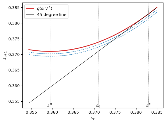
Fig. 71.1 Saving rates on constant-payoff paths#
The red curve is \(q(s; V^\ast)\), and the dashed curves are \(q(s; \bar V)\) for two values of \(\bar V\) below \(V^\ast\).
The red curve is flat at \(s^M\) and touches the 45-degree line at \(s^B\) with slope one, so convergence slows as the saving rate approaches \(s^B\).
71.3.4. Where the path starts#
The difference equation (71.7) admits a continuum of solutions with value \(V^\ast\), one for each starting point.
All of them give the first planner the same payoff, but they differ in what they ask of it.
A sequence that starts at \(s_0 = s^B\) is constant and, as we saw, violates no delay.
The first planner’s best one-period action is \(s^M\), whatever its successors do, so the no-delay condition (71.6) requires the starting point to be low enough that saving at \(s^M\) and letting the sequence start next period does not pay.
The highest starting point that passes is \(s_0 = q(s^M; V^\ast)\): with it, the sequence \(s^M, s_0, s_1, \ldots\) is itself a constant-value path, so sitting out gives exactly \(V^\ast\).
Bassetto, Huo, and Ríos-Rull select this starting point because it leaves the most capital to later planners.
The organizational equilibrium therefore starts with a saving rate about halfway from the Markov rate to \(s^B\) and raises it gradually toward \(s^B\), which is below the Ramsey planner’s long-run rate \(s^R\) for any \(\delta < 1\).
71.3.5. Transition paths#
We compare the organizational equilibrium with the Ramsey plan and the Markov equilibrium, starting from the Markov steady-state capital stock \(k^M = (s^M)^{1/(1 - \alpha)}\), as Bassetto et al. [2024] do.
The total payoff of the planner at date \(t\) is (71.1), the sum of a capital payoff and the action payoff \(V_t\).
Along the organizational path, \(V_t = V^\ast\) at every date by construction; we confirm it on a long computed path, since the saving rate converges slowly.
n_long, n_plot = 5000, 16
s_O = [s_0]
for t in range(n_long):
    s_O.append(q(s_O[-1], V_star))
s_O = np.array(s_O)

V_O = np.array([action_payoff(s_O[t:], s_B) for t in range(n_plot)])
print(f"max |V_t - V*| over {n_plot} periods = {np.abs(V_O - V_star).max():.1e}")

paths = {"organizational equilibrium": s_O[:n_plot],
         "Ramsey plan": np.r_[s_M, np.full(n_plot - 1, s_R)],
         "Markov equilibrium": np.full(n_plot, s_M)}
V_paths = {"organizational equilibrium": V_O,
           "Ramsey plan": np.r_[action_payoff([s_M], s_R),
                                np.full(n_plot - 1, action_payoff([s_R], s_R))],
           "Markov equilibrium": np.full(n_plot, action_payoff([s_M], s_M))}
c_k = α * (1 - α * β + δ * α * β) / (1 - α * β)

def capital_path(s, k_0):
    k = [k_0]
    for x in s[:-1]:
        k.append(x * k[-1]**α)
    return np.array(k)

k_M = s_M**(1 / (1 - α))
print("V_t - V* under the Ramsey plan, dates 0 and 1:",
      np.round(V_paths["Ramsey plan"][:2] - V_star, 6))
print(f"V_t - V* in the Markov equilibrium: {V_paths['Markov equilibrium'][0] - V_star:.4f}")
max |V_t - V*| over 16 periods = 1.1e-14
V_t - V* under the Ramsey plan, dates 0 and 1: [ 1.929e-03 -8.500e-05]
V_t - V* in the Markov equilibrium: -0.0437
fig, axes = plt.subplots(2, 2, figsize=(11, 7))
styles = {"organizational equilibrium": 'C3-', "Ramsey plan": 'C0--',
          "Markov equilibrium": 'k:'}
for name, s in paths.items():
    k = capital_path(s, k_M)
    axes[0, 0].plot(s, styles[name], lw=2, label=name)
    axes[0, 1].plot(k, styles[name], lw=2)
    axes[1, 0].plot(c_k * np.log(k) + V_paths[name], styles[name], lw=2)
    if name != "Markov equilibrium":
        axes[1, 1].plot(V_paths[name] - V_star, styles[name], lw=2)
for ax, title in zip(axes.flat, ["saving rate $s_t$", "capital $k_t$",
                                 "total payoff $U_t$", r"action payoff $V_t - V^*$"]):
    ax.set_title(title)
    ax.set_xlabel("period")
axes[0, 0].legend()
plt.tight_layout()
plt.show()
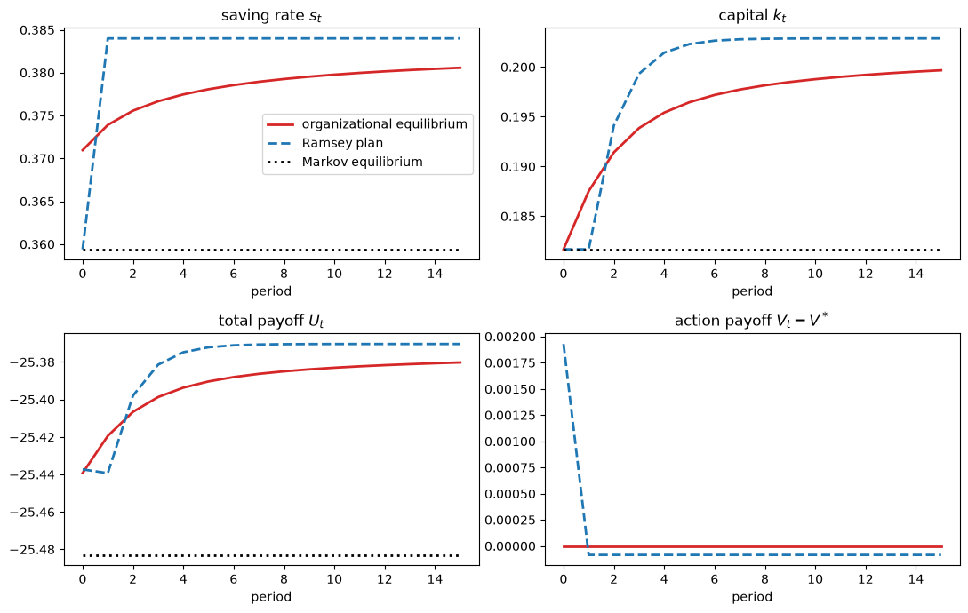
Fig. 71.2 Transition paths in three equilibria#
In the Markov equilibrium, the saving rate and capital stay at their initial levels.
The Ramsey planner saves at the Markov rate at date \(0\) and then imposes the higher rate \(s^R\) on all its successors.
In the organizational equilibrium, the date-\(0\) planner saves more than the Markov rate, so capital at date \(1\) is higher than under the Ramsey plan, and the saving rate then rises gradually.
The Ramsey plan gives the date-\(0\) planner the highest total payoff, as it must.
At date \(1\) the comparison reverses: the date-\(1\) planner inherits more capital and is asked to save less than under the Ramsey plan, so its total payoff is higher.
From date \(2\) on, capital is lower than under the Ramsey plan, and so are total payoffs.
The action payoffs, which factor out inherited capital, show the redistribution (the Markov equilibrium’s action payoff, \(0.044\) below \(V^\ast\), is left out of the last panel): an organizational equilibrium gives the first planner less than the Ramsey plan does and gives every later planner more.
71.4. Tariffs, saving, and growth#
We apply these ideas to trade policy, following Bassetto et al. [2024] and Bassetto et al. [2026].
In this application a single large player, the government, interacts with a continuum of competitive private agents.
Bassetto, Huo, and Ríos-Rull handle this setting by assuming that every sequence of government actions induces a unique competitive equilibrium that does not depend on the initial state, and by defining the government’s preferences over sequences of its own actions as its payoff in that competitive equilibrium; the definitions of the previous section then apply unchanged.
Time inconsistency now has a familiar source: private agents’ current decisions depend on expected future policy, as in Kydland and Prescott [1977], Time Inconsistency of Ramsey Plans, and Stackelberg Plans.
A tariff protects workers in the import-competing sector and raises revenue that is rebated to workers, but it lowers the return to capital, and thereby saving and growth.
A policymaker who cares about workers therefore wants high tariffs now and low tariffs later: low future tariffs encourage saving today, while today’s tariff cannot affect saving that has already been done.
71.4.1. A two-country economy#
There are two symmetric countries, home and foreign, and two goods.
Home is more productive at producing good 1, foreign at producing good 2.
In each country, a measure one of workers is attached to each sector, and capital moves freely between the two sectors.
At home, sector \(i\) produces
where \(\ell_{it}\) is labor and \(k_{it}\) capital used in sector \(i\), and the country’s aggregate capital stock \(k_t = k_{1t} + k_{2t}\) raises productivity in both sectors, an externality that makes output proportional to \(k_t\), as in an \(AK\) model.
Foreign is the mirror image of home, and the two countries start with the same capital stock.
Each government taxes imports at the rate \(\tau_t \ge 0\), and, following Bassetto et al. [2026], we assume that the foreign government matches the home tariff, so that home effectively chooses a common tariff.
Let good 2 be the numeraire at home.
Home imports good 2, so its world price is \(1/(1 + \tau_t)\), and by symmetry the world and home prices of good 1, which home exports, are also \(p_{1t} = 1/(1 + \tau_t)\).
The tariff lowers the relative price of home’s export good below its free-trade value of one.
71.4.1.1. Static equilibrium#
Equating the returns to capital in the two sectors gives the share \(\phi_t\) of capital in sector 2,
so that a higher tariff shifts capital into the import-competing sector.
Wages and the rental rate, in units of good 2, are
A final good used for consumption and investment combines the two goods with a CES aggregator with equal weights and elasticity of substitution \(\varepsilon\), and its price is
Home uses the goods in the ratio \(m_{1t} / m_{2t} = (1 + \tau_t)^{\varepsilon}\).
Because world prices of the two goods are equal, balanced trade requires home’s exports of good 1, \(Y_{1t} - m_{1t}\), to equal its imports of good 2, \(m_{2t} - Y_{2t}\).
Home collects tariff revenue \(T_t = \tau_t (m_{2t} - Y_{2t}) / (1 + \tau_t)\), which it rebates equally to the two groups of workers.
Workers do not save, so a worker in sector \(i\) consumes
where \(\psi_i(\tau)\) depends only on the tariff.
71.4.1.2. Capitalists#
Capitalists own the capital stock and rent it to firms; their consumption and investment satisfy
where \(\delta_k\) is the depreciation rate, and they maximize \(\sum_t \beta^t (c^K_t)^{1 - \sigma} / (1 - \sigma)\).
With saving rate \(s_t = k_{t+1} / (G(\tau_t) k_t)\), the Euler equation is
Iterating (71.8) forward shows that \(s_t\) depends only on future tariffs.
When \(\sigma < 1\), a higher expected return raises saving, so expected future tariffs lower saving today.
When tariffs are constant, \(s(\tau) = \left[ \beta G(\tau)^{1 - \sigma} \right]^{1/\sigma}\).
Within each period, the government sets the tariff first and capitalists then decide how much to save, so capitalists respond in the same period to any change in expected policy.
71.4.1.3. The policymaker#
The home policymaker maximizes the welfare of the average worker, \(\sum_{j \ge 0} \beta^j \tfrac12 (\log c_{1,t+j} + \log c_{2,t+j})\).
Since \(\tfrac12 (\log c_{1t} + \log c_{2t}) = \log k_t + \chi(\tau_t)\), with \(\chi(\tau) = \tfrac12 [\log \psi_1(\tau) + \log \psi_2(\tau)]\), and \(\log k_{t+1} = \log k_t + \log s_t + \log G(\tau_t)\), the policymaker’s payoff separates into a capital payoff and an action payoff:
Two functions of the tariff alone, worker welfare \(\chi(\tau)\) and the gross return \(G(\tau)\), summarize everything that the static equilibrium contributes to the dynamic policy problem.
We use the parameter values of Bassetto et al. [2024], with a model period of seven years, and set \(\sigma = 0.5\), the value used by Bassetto et al. [2026].
TariffModel = namedtuple('TariffModel', ('α', 'β', 'δ_k', 'ε', 'A', 'σ'))

def create_tariff_model(α=0.33, β=0.7, δ_k=0.65, ε=1.1, A=3.5, σ=0.5):
    return TariffModel(α=α, β=β, δ_k=δ_k, ε=ε, A=A, σ=σ)

def static(τ, model):
    """
    Worker welfare χ(τ), the gross return G(τ), and the consumption of the two
    groups of workers per unit of capital, ψ_1(τ) and ψ_2(τ).
    """
    α, β, δ_k, ε, A, σ = model
    ϕ = 1 / (1 + (A / (1 + τ))**(1 / (1 - α)))
    p_1 = 1 / (1 + τ)
    Y_1, Y_2 = A * (1 - ϕ)**α, ϕ**α
    P = (0.5 * p_1**(1 - ε) + 0.5)**(1 / (1 - ε))
    m_2 = (Y_1 + Y_2) / (1 + (1 + τ)**ε)           # balanced trade
    revenue = τ / (1 + τ) * (m_2 - Y_2)
    ψ_1 = ((1 - α) * p_1 * Y_1 + revenue / 2) / P
    ψ_2 = ((1 - α) * Y_2 + revenue / 2) / P
    χ = 0.5 * (np.log(ψ_1) + np.log(ψ_2))
    G = α * ϕ**(α - 1) / P + 1 - δ_k
    return χ, G, ψ_1, ψ_2

def χ(τ, model):
    return static(τ, model)[0]

def G(τ, model):
    return static(τ, model)[1]

def H(τ, s, model):
    β = model.β
    return χ(τ, model) + β / (1 - β) * (np.log(s) + np.log(G(τ, model)))

def s_const(τ, model):
    "The saving rate when the tariff is τ forever."
    return (model.β * G(τ, model)**(1 - model.σ))**(1 / model.σ)

model = create_tariff_model()
71.4.2. Markov and best constant tariffs#
From (71.8), today’s saving rate depends only on future tariffs.
A Markov policymaker, who takes future tariffs as given, therefore takes today’s saving rate as given and chooses
The best constant tariff instead takes into account that a permanently lower tariff raises the saving rate \(s(\tau)\); substituting \(s(\tau)\) into \(H\) gives, up to a constant,
which puts \(1/\sigma\) times as much weight on the return to capital.
def argmax(f, lo=0.0, hi=1.0):
    return minimize_scalar(lambda τ: -f(τ), bounds=(lo, hi), method='bounded',
                           options={'xatol': 1e-10}).x

def markov_tariff(model):
    β = model.β
    return argmax(lambda τ: χ(τ, model) + β / (1 - β) * np.log(G(τ, model)))

def best_constant_tariff(model):
    β, σ = model.β, model.σ
    return argmax(lambda τ: χ(τ, model) + β / (σ * (1 - β)) * np.log(G(τ, model)))

τ_M, τ_B = markov_tariff(model), best_constant_tariff(model)
H_B = H(τ_B, s_const(τ_B, model), model)
V_markov = H(τ_M, s_const(τ_M, model), model) / (1 - model.β)
V_best = H_B / (1 - model.β)
print(f"Markov tariff {100 * τ_M:.1f} percent, best constant tariff {100 * τ_B:.1f} percent")

ψ_free, ψ_markov = static(0.0, model)[2:], static(τ_M, model)[2:]
print("consumption at the Markov tariff relative to free trade: export-sector workers "
      f"{ψ_markov[0] / ψ_free[0]:.3f}, import-sector workers {ψ_markov[1] / ψ_free[1]:.3f}")
Markov tariff 24.4 percent, best constant tariff 0.4 percent
consumption at the Markov tariff relative to free trade: export-sector workers 0.938, import-sector workers 1.581
τ_grid = np.linspace(0, 0.5, 200)
fig, axes = plt.subplots(1, 2, figsize=(11, 4))
axes[0].plot(100 * τ_grid, [χ(x, model) - χ(0, model) for x in τ_grid], lw=2)
axes[0].set_title(r"worker welfare $\chi(\tau) - \chi(0)$")
axes[1].plot(100 * τ_grid, [G(x, model) for x in τ_grid], lw=2)
axes[1].set_title(r"gross return to capital $G(\tau)$")
for ax in axes:
    ax.axvline(100 * τ_B, color='C2', ls='--', lw=1, label=r"best constant tariff $\tau^B$")
    ax.axvline(100 * τ_M, color='C3', ls=':', lw=1.5, label=r"Markov tariff $\tau^M$")
    ax.set_xlabel("tariff (percent)")
axes[0].legend()
plt.tight_layout()
plt.show()
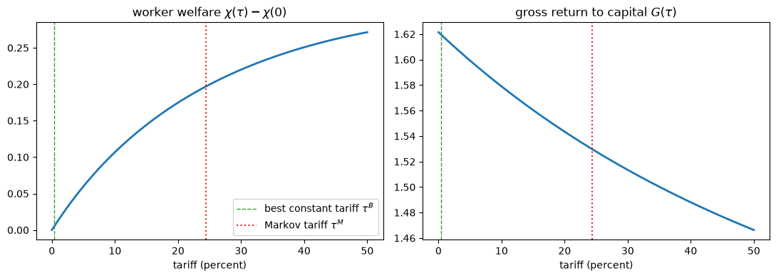
Fig. 71.3 Worker welfare and capital returns#
The tariff raises worker welfare over the whole range shown.
It raises the consumption of the lower-paid workers in the import-competing sector, through their wage and the rebated revenue, by much more in proportion than it lowers the consumption of workers in the export sector: at the Markov tariff, by 58 percent against 6 percent.
It lowers the return to capital throughout.
The Markov policymaker, who ignores how expected tariffs affect saving, chooses a high tariff; the best constant tariff is close to free trade.
71.4.3. Ramsey plan and plans sustained by Markov reversion#
A Ramsey planner at date \(0\) chooses the whole sequence of tariffs, taking into account the Euler equations (71.8).
Saving at date \(t\) depends only on tariffs after date \(t\), so the date-\(0\) tariff affects no saving rate, and the planner chooses \(\tau_0 = \tau^M\); from date \(1\) on, it lowers tariffs to encourage saving at earlier dates.
We compute the Ramsey plan by optimizing over tariffs for \(N\) periods, after which the tariff is constant.
Given a tariff sequence, we compute saving rates backward from the steady state using (71.8), and action payoffs \(V_t = \sum_{j \ge 0} \beta^j H(\tau_{t+j}, s_{t+j})\) backward from the constant tail.
def saving_rates(τ, model):
    "Saving rates for tariffs τ_0, ..., τ_N, with τ_N kept forever."
    β, σ = model.β, model.σ
    s = np.empty(len(τ))
    s[-1] = s_const(τ[-1], model)
    for t in range(len(τ) - 2, -1, -1):
        ratio = (β * G(τ[t + 1], model)**(1 - σ))**(-1 / σ) * (1 - s[t + 1])   # (1 - s_t) / s_t
        s[t] = 1 / (1 + ratio)
    return s

def action_payoffs(τ, model):
    "Action payoffs V_0, ..., V_N for tariffs τ_0, ..., τ_N, with τ_N kept forever."
    β = model.β
    s = saving_rates(τ, model)
    V = np.empty(len(τ))
    V[-1] = H(τ[-1], s[-1], model) / (1 - β)
    for t in range(len(τ) - 2, -1, -1):
        V[t] = H(τ[t], s[t], model) + β * V[t + 1]
    return V

N = 25
res = minimize(lambda τ: -action_payoffs(τ, model)[0], np.full(N + 1, 0.1),
               bounds=[(0, 1)] * (N + 1), method='L-BFGS-B')
τ_R = res.x
V_R = action_payoffs(τ_R, model)
print("Ramsey tariffs (percent):", np.round(100 * τ_R[:6], 1))
print(f"action payoffs: V_0 = {V_R[0]:.4f}, V_1 = {V_R[1]:.4f}, V_N = {V_R[-1]:.4f};  "
      f"V* = {V_best:.4f}, V_M = {V_markov:.4f}")
print(f"smallest V_t - V_M along the Ramsey plan: {(V_R - V_markov).min():.4f}")
Ramsey tariffs (percent): [24.4 14.   6.1  0.1  0.   0. ]
action payoffs: V_0 = 1.6211, V_1 = 1.6048, V_N = 1.5370;  V* = 1.5371, V_M = 1.2868
smallest V_t - V_M along the Ramsey plan: 0.2502
The Ramsey plan starts at the Markov tariff and reaches free trade within a few periods.
Free trade is a corner: we restrict tariffs to be nonnegative, as Bassetto et al. [2026] do, and without that restriction the Ramsey plan would subsidize imports from period 4 on.
The plan gives the date-\(0\) policymaker a higher action payoff than any later one, so it violates no restarting.
A sustainable plan in the sense of Chari and Kehoe [1990], the subject of Sustainable Plans for a Calvo Model, can be supported by the threat that any deviation triggers permanent reversion to the Markov equilibrium.
After a deviation, capitalists expect Markov tariffs from the next period on and save at the Markov rate, so the best deviation yields exactly the Markov action payoff \(V^M\).
A tariff path can therefore be sustained by Markov reversion if and only if \(V_t \ge V^M\) at every date, and the best such path maximizes \(V_0\) subject to these constraints.
Every Ramsey continuation is worth more than the Markov equilibrium, as the last line printed above shows, so the constraints are slack and the best path sustained by Markov reversion is the Ramsey plan.
The best sustainable plan in the sense of Sustainable Plans for a Calvo Model, which uses the worst subgame-perfect equilibrium as the punishment, is therefore also the Ramsey plan.
71.4.4. Organizational equilibrium tariffs#
Along an organizational equilibrium, the action payoff is the same at every date.
We take that value to be \(V^\ast = H(\tau^B, s^B)/(1 - \beta)\), the value of the best constant tariff, as Bassetto et al. [2026] do.
With a competitive private sector, the general results that make \(V^\ast\) the highest constant value in the growth model do not apply directly, so this choice must be checked in each application; here a numerical search over tariff paths that repeat every two, three, or four periods finds none that gives every policymaker more than \(V^\ast\).
A constant action payoff requires \(H(\tau_t, s_t) = H^B \equiv H(\tau^B, s^B)\) at every date.
Solving this equation for the saving rate gives the saving rate that a tariff \(\tau\) must induce,
and the Euler equation (71.8) then links successive tariffs:
For a given \(\tau_t\), this equation has a root \(\tau_{t+1}\) between \(\tau^B\) and \(\tau_t\) and another at a much higher tariff; the first defines the transition map \(\tau_{t+1} = \mathcal{T}(\tau_t)\), which has the fixed point \(\tau^B\).
A high tariff today must be followed by a tariff low enough tomorrow to induce the saving rate that keeps \(H(\tau_t, s_t) = H^B\).
The no-delay condition requires \(\tau_0 \ge \mathcal{T}(\tau^M)\): a policymaker who sat out would choose \(\tau^M\), and sitting out pays if the path starts with a lower tariff.
As in the growth model, we select the lowest tariff that satisfies it, \(\tau_0 = \mathcal{T}(\tau^M)\), as Bassetto et al. [2026] do; with it, the sequence \(\tau^M, \tau_0, \tau_1, \ldots\) is itself a path of constant action payoff, so sitting out gains nothing.
def s_org(τ, H_B, model):
    "The saving rate that keeps H(τ, s) equal to H_B."
    β = model.β
    return np.exp((1 - β) / β * (H_B - χ(τ, model)) - np.log(G(τ, model)))

def transition(τ, τ_B, H_B, model):
    "Next period's tariff on a path whose action payoff is constant at H_B / (1 - β)."
    if τ <= τ_B + 1e-8:
        return τ_B
    β, σ = model.β, model.σ
    s = s_org(τ, H_B, model)
    lhs = ((1 - s) / s)**(-σ)
    f = lambda τ_next: (β * G(τ_next, model)**(1 - σ)
                        * (1 - s_org(τ_next, H_B, model))**(-σ) - lhs)
    return brentq(f, τ_B, τ)                 # the root between τ_B and τ

𝒯 = lambda τ: transition(τ, τ_B, H_B, model)

τ_O = [𝒯(τ_M)]
for t in range(400):
    τ_O.append(𝒯(τ_O[-1]))
τ_O = np.array(τ_O)
V_org = action_payoffs(τ_O, model)
print("organizational tariffs (percent):", np.round(100 * τ_O[:6], 1))
print(f"max |V_t - V*| over the first 25 periods = {np.abs(V_org[:25] - V_best).max():.1e}")

ratio = ((model.β * G(τ_O[0], model)**(1 - model.σ))**(-1 / model.σ)
         * (1 - s_org(τ_O[0], H_B, model)))
s_minus = 1 / (1 + ratio)          # saving at date -1 if the path starts one period later
print(f"gain from sitting out at date 0: H(τ_M, s_-1) - H_B = {H(τ_M, s_minus, model) - H_B:.1e}")
print(f"slope of the transition map at τ_M: {(𝒯(τ_M) - 𝒯(τ_M - 1e-6)) / 1e-6:.4f}, "
      f"near τ_B: {(𝒯(τ_B + 2e-3) - 𝒯(τ_B + 1e-3)) / 1e-3:.4f}")
print(f"tariff after 20 periods {100 * τ_O[20]:.1f} percent, after 100 periods "
      f"{100 * τ_O[100]:.1f} percent")
organizational tariffs (percent): [14.2 11.6 10.   8.9  8.1  7.4]
max |V_t - V*| over the first 25 periods = 5.5e-13
gain from sitting out at date 0: H(τ_M, s_-1) - H_B = -2.6e-15
slope of the transition map at τ_M: 0.0000, near τ_B: 0.9976
tariff after 20 periods 3.8 percent, after 100 periods 1.4 percent
The action payoff is constant along the path, and the first policymaker is exactly indifferent between starting the organizational path and sitting out.
Like \(q\) in the growth model, the transition map is flat at the Markov policy and has slope one at the best constant policy, so liberalization is fast at first and then very slow: with seven-year periods, the tariff is still 3.8 percent after 140 years.
n_plot = 20
fig, axes = plt.subplots(1, 2, figsize=(12, 4.5))
grid_τ = np.linspace(τ_B, τ_M, 100)
axes[0].plot(100 * grid_τ, [100 * 𝒯(x) for x in grid_τ], 'C3', lw=2,
             label=r"$\mathcal{T}(\tau)$")
axes[0].plot(100 * grid_τ, 100 * grid_τ, 'k', lw=0.8, label="45-degree line")
axes[0].set_xlabel(r"current tariff $\tau_t$ (percent)")
axes[0].set_ylabel(r"next tariff $\tau_{t+1}$ (percent)")
axes[0].legend()
axes[1].plot(100 * τ_O[:n_plot], 'C3-o', ms=4, lw=2, label="organizational equilibrium")
axes[1].plot(100 * τ_R[:n_plot], 'C0--s', ms=4, lw=2,
             label="Ramsey plan = best plan sustained by Markov reversion")
axes[1].plot(np.full(n_plot, 100 * τ_M), 'k:', lw=2, label="Markov equilibrium")
axes[1].axhline(100 * τ_B, color='gray', lw=0.8)
axes[1].set_xlabel("period (seven years)")
axes[1].set_ylabel("tariff (percent)")
axes[1].legend()
plt.tight_layout()
plt.show()
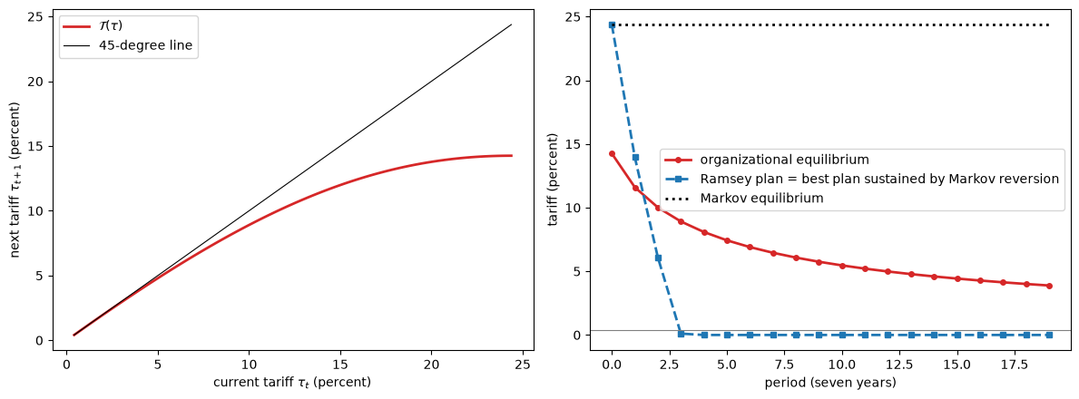
Fig. 71.4 Tariff transition map and tariff paths#
The transition map lies below the 45-degree line, so tariffs fall at every date, by a lot when they are high and by little near \(\tau^B\).
The organizational equilibrium starts well below the Markov tariff and liberalizes gradually, a pattern that Bassetto et al. [2024] compare with the decline of the world average tariff after 1950.
The Ramsey plan liberalizes much faster, but only because its first policymaker can commit its successors.
71.4.5. Temporary protectionist shocks#
The off-path behavior of the two cooperative equilibria differs sharply.
Suppose that at date 10 an unexpected shock sets the tariff to 10 percent, as in an example of Bassetto et al. [2026].
The Ramsey plan, sustained by the threat of permanent reversion, then switches to \(\tau^M\) forever.
In the organizational equilibrium, the transition map still applies: the next tariff is \(\mathcal{T}(0.1)\), and liberalization resumes from there.
t_shock, τ_shock, n_plot = 10, 0.1, 30
τ_O_shock = list(τ_O[:t_shock]) + [τ_shock]
while len(τ_O_shock) < n_plot:
    τ_O_shock.append(𝒯(τ_O_shock[-1]))
τ_S_shock = np.r_[τ_R[:t_shock], τ_shock, np.full(n_plot - t_shock - 1, τ_M)]
t_back = np.argmin(np.abs(τ_O - 𝒯(τ_shock)))
print(f"tariff after the shock: {100 * 𝒯(τ_shock):.1f} percent, the undisturbed path's "
      f"tariff at period {t_back}")

fig, ax = plt.subplots()
ax.plot(100 * np.array(τ_O_shock), 'C3-o', ms=4, lw=2, label="organizational equilibrium")
ax.plot(100 * τ_S_shock, 'C0--s', ms=4, lw=2, label="plan sustained by Markov reversion")
ax.plot(np.full(n_plot, 100 * τ_M), 'k:', lw=2, label="Markov equilibrium")
ax.axvline(t_shock, color='gray', ls=':', lw=1)
ax.set_xlabel("period (seven years)")
ax.set_ylabel("tariff (percent)")
ax.legend(loc='upper right', bbox_to_anchor=(1, 0.88))
plt.show()
tariff after the shock: 8.9 percent, the undisturbed path's tariff at period 3
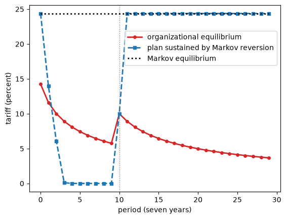
Fig. 71.5 Tariffs after a protectionist shock#
One period after the shock, the organizational tariff is back at the level that the undisturbed path reached at period 3, so the shock delays liberalization by eight periods, about 56 years, but does not change where liberalization ends up.
In the plan sustained by Markov reversion, a one-period disturbance permanently destroys cooperation, a self-inflicted punishment that later policymakers would want to renegotiate.
71.4.6. A quantitative version#
Bassetto et al. [2026] replace the two-sector static block with a model of the G7 economies with 30 sectors, input-output linkages, and trade in final and intermediate goods, disciplined by the World Input-Output Database and KLEMS data.
Because aggregate capital enters each firm’s technology as an externality, the static equilibrium is again proportional to world capital, and the dynamic policy problem depends on the static block only through \(\chi(\tau)\) and \(G(\tau)\), as in (71.9).
That separability lets them compute \(\chi(\tau)\) and \(G(\tau)\) by exact-hat algebra [Dekle et al., 2008] from observed trade shares, without separately estimating technologies and tastes.
They find a Markov tariff of about 12 percent and a best constant tariff of about 1.3 percent, and that the tariff raises worker welfare mainly by compressing consumption differences across sectors through the equal rebate of tariff revenue.
71.5. Connections to other lectures#
Organizational equilibrium adds a fourth equilibrium concept to the three that several lectures in this section study.
Gradualism in Self-Enforcing Trade Agreements explains gradual liberalization differently, as a feature of efficient self-enforcing agreements between countries of different size that are sustained by the threat of a permanent trade war [Bond and Park, 2002], the kind of cooperation whose fragility to a single deviation Tariffs, saving, and growth illustrates.
Time Inconsistency of Ramsey Plans computes a Ramsey plan, a Markov perfect equilibrium, and a constrained-to-constant-growth Ramsey plan in a model of inflation; the last is the analogue of the best constant action, and an organizational equilibrium converges to it but, because of no delay, does not start there.
Sustainable Plans for a Calvo Model supports good outcomes in the same model with Abreu’s severe stick-and-carrot punishments [Abreu, 1988], whereas an organizational equilibrium can use punishments proportional to the deviation and gives every policymaker the same action payoff.
Credible Government Policies in a Model of Chang computes the values of credible plans by iterating on a set-to-set operator in the manner of Abreu et al. [1986] and Abreu et al. [1990], an iteration that Bassetto, Huo, and Ríos-Rull cannot use because their symmetry requirement, that every continuation give the same value as the whole equilibrium, is an equality constraint.
Stackelberg Plans, Optimal Taxation with State-Contingent Debt, and Competitive Equilibria of a Model of Chang make Ramsey plans recursive by carrying promised values or promised private-sector decisions as state variables, which is needed because, as in the tariff model, later actions are chosen partly to shape earlier private decisions.
Accounting for Monetary and Fiscal Policy studies a government that cannot fully commit and whose economy switches endogenously between monetary-dominant and fiscal-dominant regimes; organizational equilibrium offers a way to think about how institutions that discipline such a government might be built up over time.
International Lending with Moral Hazard and Risk of Repudiation and Capital Flows Under Moral Hazard study lending sustained by the threat of permanent exclusion into autarky, a punishment of the same permanent kind as reversion to the Markov equilibrium in Tariffs, saving, and growth.
71.6. Exercises#
Exercise 71.1
In the growth model of A savings problem with present bias, the organizational equilibrium converges to the best constant saving rate \(s^B\), which lies below the Ramsey planner’s long-run rate \(s^R = \alpha\beta\).
For \(\delta \in \{0.5, 0.7, 0.9, 0.95, 0.99\}\), holding \(\alpha = 0.4\) and \(\beta = 0.96\) fixed, compute \(s^M\), the first organizational saving rate \(s_0 = q(s^M; V^\ast)\), \(s^B\), and \(s^R\), and the numbers of periods that the organizational path takes to close half and 90 percent of the gap between \(s_0\) and \(s^B\).
How do the long-run gap \(s^R - s^B\) and the speed of convergence depend on \(\delta\)?
Solution
α_g, β_g = 0.4, 0.96

def periods_to_close(fraction, s_start, s_target, V, δ):
    "Periods until the organizational path closes the given fraction of the gap."
    s, t = s_start, 0
    while s_target - s > (1 - fraction) * (s_target - s_start):
        s = q(s, V, α_g, β_g, δ)
        t += 1
    return t

print("  δ      s_M      s_0      s_B      s_R    s_R - s_B   periods to close 50% and 90%")
for δ_i in [0.5, 0.7, 0.9, 0.95, 0.99]:
    s_M_i, s_B_i, s_R_i = benchmarks(α_g, β_g, δ_i)
    V_i = action_payoff([s_B_i], s_B_i, α_g, β_g, δ_i)
    s_0_i = q(s_M_i, V_i, α_g, β_g, δ_i)
    t_50, t_90 = [periods_to_close(f, s_0_i, s_B_i, V_i, δ_i) for f in (0.5, 0.9)]
    print(f"{δ_i:5.2f}  {s_M_i:7.4f}  {s_0_i:7.4f}  {s_B_i:7.4f}  {s_R_i:7.4f}"
          f"  {s_R_i - s_B_i:10.5f}  {t_50:6d}  {t_90:6d}")
  δ      s_M      s_0      s_B      s_R    s_R - s_B   periods to close 50% and 90%
 0.50   0.2376   0.2970   0.3748   0.3840     0.00923       5      46
 0.70   0.3038   0.3394   0.3800   0.3840     0.00401       4      39
 0.90   0.3594   0.3710   0.3830   0.3840     0.00105       4      35
 0.95   0.3719   0.3777   0.3835   0.3840     0.00050       4      35
 0.99   0.3816   0.3828   0.3839   0.3840     0.00010       4      34
As \(\delta\) rises toward one, the present bias weakens, and \(s^M\), \(s_0\), and \(s^B\) all approach the Ramsey rate \(s^R\), but \(s^B < s^R\) for every \(\delta < 1\).
Whatever \(\delta\), the organizational path closes half of its initial gap in four or five periods but needs 34 to 46 periods to close 90 percent of it, because \(q(\cdot; V^\ast)\) has slope one at \(s^B\).
Convergence is slightly faster when the present bias is weak.
Exercise 71.2
The difference equation (71.7) with \(\bar V = V^\ast\) has a solution for each starting point \(\hat s \in [s^M, s^B]\), and all of them give the first planner the action payoff \(V^\ast\).
For a grid of starting points, compute the first planner’s gain from sitting out, \(V(s^M, \hat s, s_1, \ldots) - V^\ast\), and confirm that the no-delay condition (71.6) holds exactly when \(\hat s \le q(s^M; V^\ast)\).
Use (71.7) to show that the gain equals \(\beta (1 - \delta) \left[ \log\left(1 - q(s^M; V^\ast)\right) - \log(1 - \hat s) \right]\).
Hint: compute each path for many periods, and append \(s^B\) as the constant tail.
Solution
def constant_value_path(s_start, n=5000):
    s = [s_start]
    for t in range(n):
        s.append(q(s[-1], V_star))
    return s

starts = np.linspace(s_M, s_B, 9)
gains = [action_payoff([s_M] + constant_value_path(x), s_B) - V_star for x in starts]
formula = β * (1 - δ) * (np.log(1 - q(s_M, V_star)) - np.log(1 - starts))
print(f"max |computed gain - formula| = {np.abs(np.array(gains) - formula).max():.1e}")

fig, ax = plt.subplots()
ax.plot(starts, gains, 'o-', lw=2)
ax.axhline(0, color='k', lw=0.8)
ax.axvline(q(s_M, V_star), color='C3', ls=':', label=r"$q(s^M; V^*)$")
ax.set_xlabel(r"starting saving rate $\hat s$")
ax.set_ylabel("gain from sitting out")
ax.legend()
plt.tight_layout()
plt.show()
max |computed gain - formula| = 8.3e-15
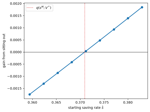
The gain from sitting out is negative for low starting points, zero at \(\hat s = q(s^M; V^\ast)\), and positive above it, where the first planner would rather save at the Markov rate and let its successor start the sequence.
For the formula, write \(V_t\) for the action payoff of the sequence \(s^M, \hat s, s_1, \ldots\) from date \(t\) on, so that \(V_1 = V^\ast\).
Subtracting \(\beta V_1\) from \(V_0\) as in the derivation of (71.7) gives \(V_0 - \beta V^\ast = \log(1 - s^M) + \frac{\delta\alpha\beta}{1 - \alpha\beta} \log s^M - \beta(1 - \delta) \log(1 - \hat s)\).
By the definition of \(q\), the first two terms on the right side equal \((1 - \beta) V^\ast + \beta(1 - \delta) \log\left(1 - q(s^M; V^\ast)\right)\).
Substituting gives \(V_0 - V^\ast = \beta (1 - \delta) \left[ \log\left(1 - q(s^M; V^\ast)\right) - \log(1 - \hat s) \right]\), which is positive exactly when \(\hat s > q(s^M; V^\ast)\) and rises with \(\hat s\).
Exercise 71.3
In the tariff model of Tariffs, saving, and growth, time inconsistency arises because capitalists’ saving responds to expected returns.
For \(\sigma \in \{0.3, 0.5, 0.7, 1.0\}\), compute the Markov tariff \(\tau^M\), the best constant tariff \(\tau^B\), and the first organizational tariff \(\mathcal{T}(\tau^M)\).
Explain why the three coincide when \(\sigma = 1\).
Solution
print("   σ    τ_M (%)   τ_B (%)   T(τ_M) (%)")
for σ_i in [0.3, 0.5, 0.7, 1.0]:
    model_i = create_tariff_model(σ=σ_i)
    τ_M_i, τ_B_i = markov_tariff(model_i), best_constant_tariff(model_i)
    H_B_i = H(τ_B_i, s_const(τ_B_i, model_i), model_i)
    τ_0_i = transition(τ_M_i, τ_B_i, H_B_i, model_i)
    print(f"{σ_i:5.1f}  {100 * τ_M_i:8.2f}  {100 * τ_B_i:8.2f}  {100 * τ_0_i:10.2f}")
   σ    τ_M (%)   τ_B (%)   T(τ_M) (%)
  0.3     24.37      0.00       12.48
  0.5     24.37      0.41       14.25
  0.7     24.37     10.72       19.03
  1.0     24.37     24.37       24.37
The Markov tariff does not depend on \(\sigma\), because a Markov policymaker takes the saving rate as given.
The best constant tariff rises with \(\sigma\), because the saving rate responds less to the return to capital, and so does the first organizational tariff.
With \(\sigma = 0.3\), the best constant tariff is at the corner \(\tau^B = 0\).
With \(\sigma = 1\), capitalists save the constant fraction \(\beta\) of their wealth whatever the return, so expected tariffs do not affect saving, there is no time inconsistency, and the Markov, best constant, and organizational tariffs coincide.