
32. Policy Counterfactuals in a New Keynesian Economy#
32.1. Overview#
Policy Counterfactuals from Impulse Responses and Policy Regimes and the Lucas Critique apply the method of McKay and Wolf [2023] to a market for a single good.
In that market, every policy rule that we studied delivers a unique equilibrium, and the government has a single instrument, a tax.
Caravello et al. [2026] extend McKay and Wolf’s results in directions that the market cannot illustrate.
This lecture studies those extensions in the textbook New Keynesian model of Galí [2015] and Woodford [2003], augmented, as in Caravello et al. [2026], with a government budget constraint and a demand for money.
The lecture
shows that an interest-rate peg, which in this economy admits many equilibria, leaves a fingerprint on McKay and Wolf’s objects: a direction of policy shocks that moves inflation but not the interest rate,
uses responses to shocks to an active Taylor rule to compute every equilibrium under a peg, and selects one by monetary dominance or by the fiscal theory of the price level,
evaluates a rule for the money supply using evidence about shocks to an interest-rate rule,
evaluates forward guidance under imperfect commitment, an interest-rate peg that ends at a random date,
computes optimal policy under commitment and under discretion from the same objects, following Hebden and Winkler [2026], and
compares all of these counterfactuals with a common loss function.
Throughout, the econometrician knows only the responses, under the baseline Taylor rule, to a cost-push shock and to contemporaneous and news shocks to the rule.
For the fiscal-theory selection she also uses the government’s budget constraint and the discount factor.
We use the model’s equations only to check her answers.
The questions are old ones.
Sargent and Wallace [1975] showed that, in a rational expectations model, an interest-rate rule can leave the price level indeterminate while a money-supply rule determines it, and Leeper [1991] showed that which authority pins down the price level depends on the mix of active and passive monetary and fiscal policies.
The new element is that McKay and Wolf’s sufficient statistics, measured in one regime, answer these questions for another.
We use the following imports.
import numpy as np
import matplotlib.pyplot as plt
32.2. The economy#
Output \(y_t\), inflation \(\pi_t\), and the nominal interest rate \(r_t\) satisfy an IS curve and a Phillips curve,
where \(e_t\) is a cost-push shock that follows the ARMA(1,1) process \(e_t = 0.7 e_{t-1} + u_t + 0.4 u_{t-1}\).
The price level is \(p_t = p_{t-1} + \pi_t\), with \(p_{-1} = 0\), and the demand for money is
The government’s debt \(b_t\) evolves according to
where \(\tau_t\) is taxes and \(\bar b / \bar y\) is the steady-state ratio of debt to output.
All variables are deviations from a steady state.
In the baseline, the central bank follows the Taylor rule
with \(\phi_\pi > 1\), and the fiscal authority adjusts taxes to keep debt from exploding.
In the language of Leeper [1991], monetary policy is active and fiscal policy passive: the regime is one of monetary dominance.
Households are Ricardian, so the timing of taxes does not affect \((y, \pi, r)\), and we need not track taxes and debt in this regime.
The parameters follow Appendix A.5 of Caravello et al. [2026]: a quarterly discount factor \(\beta = 0.99^{1/4}\), which implies a real interest rate of 1 percent a year, \(\gamma = 1\), \(\kappa = 0.02\), \(\rho_r = 0.8\), and \(\phi_\pi = 1.7\).
Write \(x\) for the stacked paths of \((y, \pi, r, p, m)\).
As in Policy Counterfactuals from Impulse Responses, we stack the equations for \(t = 0, \ldots, T-1\) into one linear system, with the convention that the forward-looking variables return to the steady state by date \(T\).
Under the baseline rule, the paths that follow a cost-push shock at date 0 and a sequence \(\nu\) of shocks to the rule, all known at date 0, are
where \(x_A\) is the response to the cost-push shock and column \(\ell\) of \(\Theta_\nu\) is the response to news, received at date 0, of a unit shock to the rule at date \(\ell\).
The pair \((x_A, \Theta_\nu)\) is the econometrician’s set of sufficient statistics.
β, γ, κ = 0.99**0.25, 1.0, 0.02     # discount factor, inverse IES, slope of the Phillips curve
ρ_r, φ_π = 0.8, 1.7                 # baseline Taylor rule
η = 0.3                             # interest semi-elasticity of money demand
T = 300                             # length of the stacked paths

e = 0.7 ** np.arange(T)             # cost-push shock after u_0 = 1
e[1:] += 0.4 * 0.7 ** np.arange(T - 1)

I, O = np.eye(T), np.zeros((T, T))
lead, lag = np.eye(T, k=1), np.eye(T, k=-1)    # lead @ x gives x_(t+1), lag @ x gives x_(t-1)

def private_block(γ=γ):
    """
    IS curve, Phillips curve, price level, and money demand for t = 0, ..., T-1.
    Unknowns are ordered x = (y, π, r, p, m).
    """
    IS = np.hstack([I - lead, -lead / γ, I / γ, O, O])     # y - y' + (r - π')/γ = 0
    PC = np.hstack([-κ * I, I - β * lead, O, O, O])         # π - κ y - β π' = e
    PL = np.hstack([O, -I, O, I - lag, O])                  # p - p_(-1) - π = 0
    MD = np.hstack([-I, O, η * I, -I, I])                   # m - p - y + η r = 0
    return np.vstack([IS, PC, PL, MD])

def taylor_rule(φ_π=φ_π):
    "The rows of r - ρ_r r_(-1) - (1 - ρ_r) φ_π π = ν."
    return np.hstack([O, -(1 - ρ_r) * φ_π * I, I - ρ_r * lag, O, O])

def forcing():
    "Right-hand side for the cost-push shock."
    out = np.zeros(5 * T)
    out[T:2 * T] = e
    return out

def split(x):
    "Split a stacked path into (y, π, r, p, m)."
    return [x[b * T:(b + 1) * T] for b in range(5)]

M_inv = np.linalg.inv(np.vstack([private_block(), taylor_rule()]))
x_A = M_inv @ forcing()             # response to the cost-push shock under the Taylor rule
Θ_ν = M_inv[:, 4 * T:]              # responses to date-0 news about the rule shock at each date
names = ["output $y$", "inflation $\\pi$", "interest rate $r$", "price level $p$", "money $m$"]
disc = β ** np.arange(T)
The next figure shows \(x_A\) and two columns of \(\Theta_\nu\).
H_plot = 24
fig, axes = plt.subplots(1, 3, figsize=(14, 4))
for i in range(3):
    axes[i].plot(split(x_A)[i][:H_plot], 'k', lw=2, label="cost-push shock")
    for ℓ, color in [(0, 'C0'), (8, 'C1')]:
        label = "rule shock, surprise" if ℓ == 0 else f"rule shock, news about date {ℓ}"
        axes[i].plot(split(Θ_ν[:, ℓ])[i][:H_plot], color=color, lw=2, label=label)
    axes[i].axhline(0, color='k', lw=0.5)
    axes[i].set_title(names[i])
    axes[i].set_xlabel("quarters")
axes[0].legend(fontsize=8)
plt.tight_layout()
plt.show()
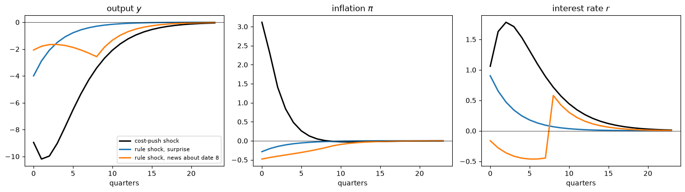
Fig. 32.1 Responses under the Taylor rule#
The Taylor rule raises the interest rate after a cost-push shock, which lowers output and moderates inflation.
A contractionary surprise to the rule lowers output and inflation.
News of a contractionary shock at date 8 lowers output and inflation at once, because both the IS curve and the Phillips curve are forward looking; until the shock arrives, the Taylor rule responds to the lower inflation by cutting the interest rate.
32.3. The fingerprint of a peg#
Consider the counterfactual peg \(r_t = 0\) for all \(t\), with fiscal policy still passive.
Substituting the Phillips curve into the IS curve shows that, with \(r_t = 0\), the vector \(z_t = (y_t, \pi_t)\) satisfies
A_peg = np.array([[1 + κ / (γ * β), -1 / (γ * β)],
                  [-κ / β, 1 / β]])
μ_peg, V_peg = np.linalg.eig(A_peg)
μ_s = μ_peg.min()                          # the stable eigenvalue
print("eigenvalues of A:", np.round(μ_peg, 4))
eigenvalues of A: [1.1533 0.8692]
One eigenvalue, \(\mu_s\), is inside the unit circle.
Both \(y_t\) and \(\pi_t\) are free to jump, so adding to any bounded equilibrium a multiple of \(\mu_s^t v_s\), where \(v_s\) is the eigenvector of \(\mu_s\), gives another: under the peg, equilibrium is indeterminate.
The multiple is a sunspot, a self-fulfilling revision of expected inflation and output that the peg does nothing to oppose.
How does this appear in McKay and Wolf’s objects?
Any path of \((y, \pi, r)\) that satisfies the IS and Phillips curves is the equilibrium under the Taylor rule for the rule shocks \(\nu_t = r_t - \rho_r r_{t-1} - (1 - \rho_r) \phi_\pi \pi_t\), so every equilibrium under the peg takes the form (32.5) for some \(\nu\) that keeps the interest rate at zero.
Under the peg these shocks are \(\nu_t = -(1 - \rho_r) \phi_\pi \pi_t = -0.34\, \pi_t\).
Two different equilibria under the peg have the same interest-rate path, so their difference is produced by shocks \(\nu_h\) with \(\Theta_{r,\nu}\, \nu_h = 0\), where \(\Theta_{r,\nu}\) collects the interest-rate rows of \(\Theta_\nu\).
These shocks exactly offset the Taylor rule’s response to a sunspot, leaving the interest rate unchanged, and they decay at the rate \(\mu_s\).
So \(\Theta_{r,\nu}\) is singular.
In our truncated system, its restriction to the first \(K\) dates is nearly singular, with a smallest singular value of the order of \(\mu_s^K\).
K = 120                                    # the peg is imposed on dates 0, ..., K-1
Θ_r = Θ_ν[2 * T:3 * T]
_, sing_vals, V_t = np.linalg.svd(Θ_r[:K, :K])
print("three smallest singular values:", sing_vals[-3:], f";  μ_s^K = {μ_s**K:.1e}")

ν_h = V_t[-1]                              # the direction of policy shocks with no effect on r
x_h = Θ_ν[:, :K] @ ν_h
y_h, π_h, r_h, p_h, m_h = split(x_h)
print(f"largest effect on r over the first K dates: {np.abs(r_h[:K]).max():.1e}")
print("π_(t+1)/π_t along the sunspot direction:", np.round(π_h[1:6] / π_h[:5], 4))
print("ν_t/π_t along the sunspot direction:    ", np.round(ν_h[:5] / π_h[:5], 4))
print(f"stable eigenvalue μ_s: {μ_s:.4f}")
three smallest singular values: [5.55220571e-01 5.55080118e-01 1.65993137e-07] ;  μ_s^K = 5.0e-08
largest effect on r over the first K dates: 1.6e-07
π_(t+1)/π_t along the sunspot direction: [0.8692 0.8692 0.8692 0.8692 0.8692]
ν_t/π_t along the sunspot direction:     [-0.34 -0.34 -0.34 -0.34 -0.34]
stable eigenvalue μ_s: 0.8692
One singular value is several orders of magnitude smaller than the others.
Along the corresponding direction, the interest rate does not move, inflation decays at exactly the rate \(\mu_s\), and the shocks are \(-0.34\) times inflation: these policy shocks implement the sunspot.
Caravello et al. [2026] prove the general result in their Proposition 2 (not to be confused with Proposition 2 of McKay and Wolf [2023], on optimal policy).
When a counterfactual rule \(\tilde R x = 0\) admits many equilibria, the solutions \(\nu\) of \(\tilde R (x_A + \Theta_\nu \nu) = 0\) trace out all of them.
The space of outcomes that policy can implement is a property of the private sector’s equations, not of the policy regime that generated the data.
The econometrician who has measured \(\Theta_\nu\) under an active Taylor rule therefore knows every equilibrium under the peg.
What she cannot learn from those data is which equilibrium would occur.
Cochrane [2011] makes a related point about Taylor rules: the response to inflation that rules out other equilibria operates only off the equilibrium path, so data generated by an equilibrium do not reveal it.
32.4. Monetary dominance and the fiscal theory#
Picking one equilibrium requires a criterion for equilibrium selection.
Under monetary dominance, fiscal policy stays passive, and the peg is understood as the limit of a peg that ends at a far-off date \(K\), after which the Taylor rule returns.[1]
Caravello et al. [2026] note that this selection coincides with others proposed in the literature: exact convergence to the steady state in finite time [Angeletos et al., 2026], and continuity of the equilibrium as policy crosses the boundary of determinacy [Lubik and Schorfheide, 2004].
We implement it by choosing the shocks on dates \(0, \ldots, K-1\) that keep the rate at zero, and no shocks afterward.
Under fiscal dominance, the fiscal authority keeps taxes at their steady-state level, \(\tau_t = 0\), as in the fiscal theory of the price level [Cochrane, 2023, Leeper, 1991].
Inflation then pays for the debt by revaluing the government’s nominal liabilities; the fiscal dominance of Sargent and Wallace [1981] works instead through seigniorage, which (32.3) omits.
Multiplying (32.3) by \(\beta^t\) and summing, with \(b_{-1} = 0\) and \(\tau_t = 0\), gives \(\beta^t b_t = -(\bar b / \bar y) \sum_{s=0}^t \beta^s (\pi_s - r_{s-1})\), so the transversality condition \(\lim_{t \to \infty} \beta^t b_t = 0\), and with it the present-value form of the government’s budget constraint, holds only if
with \(r_{-1} = 0\).
As long as there is nominal debt, \(\bar b \neq 0\), the debt ratio \(\bar b / \bar y\) scales out of (32.6), so its value does not matter; with \(\bar b = 0\), inflation cannot revalue the debt, the transversality condition no longer implies (32.6), and fiscal policy selects no equilibrium.
Inflation must adjust so that the ex post real return on the debt, \(r_{t-1} - \pi_t\), has zero present value.
Under the peg, (32.6) requires discounted cumulative inflation to be zero.
In McKay and Wolf’s objects, the fiscal-dominance equilibrium is the monetary-dominance equilibrium plus the multiple of the sunspot direction that satisfies (32.6).
def peg_equilibria(r_target=np.zeros(K), x_base=x_A):
    """
    Equilibria with r_t = r_target_t for t < K, starting from the baseline paths x_base:
    monetary dominance (the Taylor rule returns at date K) and fiscal dominance (the
    present-value condition holds), together with the rule shocks that implement them.
    """
    ν_md = np.linalg.solve(Θ_r[:K, :K], r_target - x_base[2 * T:2 * T + K])
    x_md = x_base + Θ_ν[:, :K] @ ν_md
    r_lag = np.concatenate([[0.0], split(x_md)[2][:-1]])
    c = -np.sum(disc * (split(x_md)[1] - r_lag)) / np.sum(disc * π_h)
    return x_md, ν_md, x_md + c * x_h, ν_md + c * ν_h

x_md, ν_md, x_fd, ν_fd = peg_equilibria()
for K_i in [60, 90, 120]:
    ν_i = np.linalg.solve(Θ_r[:K_i, :K_i], -x_A[2 * T:2 * T + K_i])
    print(f"peg for {K_i:3d} quarters, then the Taylor rule: π_0 = {split(x_A + Θ_ν[:, :K_i] @ ν_i)[1][0]:.4f}")
for label, x in [("Taylor rule", x_A), ("peg, monetary dominance", x_md),
                 ("peg, fiscal dominance", x_fd)]:
    print(f"{label:24s}: y_0 = {split(x)[0][0]:6.2f},  π_0 = {split(x)[1][0]:6.3f},  "
          f"discounted cumulative inflation = {np.sum(disc * split(x)[1]):7.3f}")
peg for  60 quarters, then the Taylor rule: π_0 = 5.5889
peg for  90 quarters, then the Taylor rule: π_0 = 5.5889
peg for 120 quarters, then the Taylor rule: π_0 = 5.5889
Taylor rule             : y_0 =  -8.95,  π_0 =  3.114,  discounted cumulative inflation =   8.320
peg, monetary dominance : y_0 =  14.37,  π_0 =  5.589,  discounted cumulative inflation =  19.843
peg, fiscal dominance   : y_0 =  -3.16,  π_0 =  2.951,  discounted cumulative inflation =  -0.000
Lengthening the peg from 60 to 120 quarters before the Taylor rule returns leaves the monetary-dominance value of \(\pi_0\) unchanged to four decimal places, as the limit that defines it requires.
The peg must nevertheless stay well short of the truncation date \(T = 300\).
Along the near-null direction, small errors from truncating the system at \(T\), and rounding errors, are amplified, so that a peg of, say, 250 quarters gives a value of \(\pi_0\) far from the limit that depends on those errors.
We check both answers against the model’s equations.
With the interest rate fixed at zero, the IS and Phillips curves alone determine \((y, \pi)\) once we impose a return to the steady state by date \(T\), which is the monetary-dominance selection of Angeletos et al. [2026].
Adding the multiple of \(\mu_s^t v_s\) that satisfies (32.6) gives the fiscal-dominance equilibrium.
IS_PC = np.block([[I - lead, -lead / γ], [-κ * I, I - β * lead]])
z_md = np.linalg.solve(IS_PC, np.concatenate([np.zeros(T), e])).reshape(2, T).T
i_s = np.argmin(np.abs(μ_peg))
sunspot = np.outer(μ_peg[i_s] ** np.arange(T), V_peg[:, i_s])
c_fd = -np.sum(disc * z_md[:, 1]) / np.sum(disc * sunspot[:, 1])
z_fd = z_md + c_fd * sunspot
for label, x, z in [("monetary dominance", x_md, z_md), ("fiscal dominance", x_fd, z_fd)]:
    gap = np.abs(np.column_stack(split(x)[:2])[:60] - z[:60]).max()
    print(f"{label:18s}: max |McKay–Wolf - model| over 60 quarters = {gap:.1e}")
for K_i in [40, 60, 90, 120]:
    ν_i = np.linalg.solve(Θ_r[:K_i, :K_i], -x_A[2 * T:2 * T + K_i])
    gap = np.abs(np.column_stack(split(x_A + Θ_ν[:, :K_i] @ ν_i)[:2])[:60] - z_md[:60]).max()
    print(f"monetary dominance, peg for {K_i:3d} quarters: max |McKay–Wolf - model| = {gap:.1e}")
monetary dominance: max |McKay–Wolf - model| over 60 quarters = 5.7e-09
fiscal dominance  : max |McKay–Wolf - model| over 60 quarters = 8.9e-07
monetary dominance, peg for  40 quarters: max |McKay–Wolf - model| = 3.5e-03
monetary dominance, peg for  60 quarters: max |McKay–Wolf - model| = 4.6e-05
monetary dominance, peg for  90 quarters: max |McKay–Wolf - model| = 1.2e-07
monetary dominance, peg for 120 quarters: max |McKay–Wolf - model| = 5.7e-09
The gaps are smallest when the peg lasts about 90 quarters.
For shorter pegs, the error from ending the peg after \(K\) dates dominates; for longer ones, rounding error, which the nearly singular system amplifies along the sunspot direction, takes over.
The lecture uses \(K = 120\), at which the gap is still only about \(2 \times 10^{-6}\) and the near-null direction is easier to see.
The next figure shows the two selected equilibria, other equilibria under the peg, and the shocks to the Taylor rule that implement the two selections.
fig, axes = plt.subplots(1, 4, figsize=(17, 4))
scale = (split(x_fd)[1][0] - split(x_md)[1][0]) / π_h[0]
for c in np.linspace(-1.5, 2.5, 9) * scale:
    for i in range(3):
        axes[i].plot(split(x_md + c * x_h)[i][:H_plot], color='0.8', lw=1)
for x, ν, color, label in [(x_md, ν_md, 'C0', "peg, monetary dominance"),
                           (x_fd, ν_fd, 'C1', "peg, fiscal dominance")]:
    for i in range(3):
        axes[i].plot(split(x)[i][:H_plot], color=color, lw=2, label=label)
    axes[3].plot(ν[:H_plot], color=color, lw=2, label=label)
for i in range(3):
    axes[i].plot(split(x_A)[i][:H_plot], 'k:', lw=2, label="Taylor rule")
    axes[i].set_title(names[i])
axes[3].set_title("shocks to the Taylor rule")
for ax in axes:
    ax.axhline(0, color='k', lw=0.5)
    ax.set_xlabel("quarters")
axes[0].legend(fontsize=8)
plt.tight_layout()
plt.show()
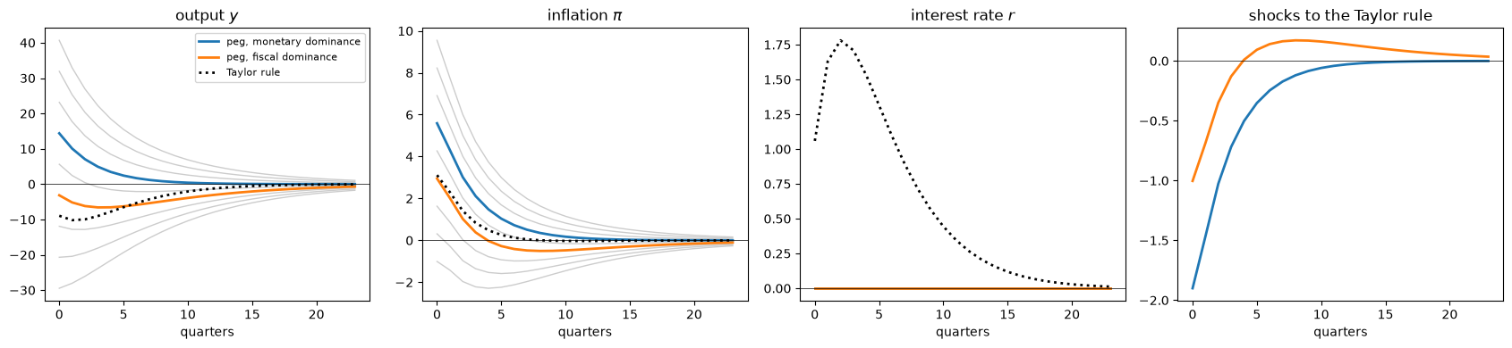
Fig. 32.2 Equilibria under an interest-rate peg#
The gray lines are other equilibria under the peg, each with a different sunspot.
The shocks in the right panel are \(-0.34\) times the inflation paths in the second panel.
Under monetary dominance, leaving the interest rate at zero after a cost-push shock raises inflation much more than the Taylor rule does, and it turns the recession into a boom.
Under fiscal dominance, inflation rises by less than under the Taylor rule, 2.95 against 3.11 on impact, and later falls below zero, so that discounted cumulative inflation is zero; output falls by a third as much on impact, \(-3.2\) against \(-9.0\), but the recession is more persistent: output bottoms out at \(-6.6\) in quarter 3, against \(-10.2\) in quarter 1 under the Taylor rule, and from quarter 6 on it is below its Taylor-rule path.
Both equilibria are implemented by shocks to an active Taylor rule in a regime of monetary dominance: in the phrase of Caravello et al. [2026], policy causal effects are portable across regimes.
Exercise 32.1 uses the same construction to study the “stepping on a rake” effect of Sims [2011], in which a higher interest rate raises inflation under fiscal dominance.
32.5. Changing the instrument#
Sargent and Wallace [1975] contrasted an interest-rate instrument with a money-supply instrument.
In their model an interest-rate peg leaves the price level indeterminate; in this economy, with sticky prices, it leaves output and inflation indeterminate too.
Caravello et al. [2026] observe that McKay and Wolf’s method covers a counterfactual rule stated in terms of an instrument other than the one that policy shocks move, provided that a private-sector relation, here the money demand (32.2), links the two.
As with the peg, \(\Theta_\nu\) describes the outcomes that policy can implement, whatever the instrument.
We evaluate the rule \(m_t = 0\), a constant money supply, and compare the smallest singular values of the matrices that map rule shocks on the first \(K\) dates into the money supply and into the interest rate.
R_m = np.hstack([O, O, O, O, I])                 # the rule m_t = 0
ν_m = np.linalg.solve(R_m @ Θ_ν, -R_m @ x_A)
x_m = x_A + Θ_ν @ ν_m
x_m_true = np.linalg.solve(np.vstack([private_block(), R_m]), forcing())
print(f"max |McKay–Wolf - model| over 100 quarters = "
      f"{max(np.abs(a[:100] - b[:100]).max() for a, b in zip(split(x_m), split(x_m_true))):.1e}")
print("   K   smallest singular value: money rule        peg")
for K_i in [60, 90, 120]:
    s_m = np.linalg.svd(Θ_ν[4 * T:4 * T + K_i, :K_i], compute_uv=False)[-1]
    s_r = np.linalg.svd(Θ_r[:K_i, :K_i], compute_uv=False)[-1]
    print(f"{K_i:4d}   {s_m:33.3f}   {s_r:9.1e}")
print("money along the sunspot direction, relative to date 0:", np.round(m_h[:5] / m_h[0], 4))
max |McKay–Wolf - model| over 100 quarters = 3.6e-13
   K   smallest singular value: money rule        peg
  60                               0.444     7.4e-04
  90                               0.444     1.1e-05
 120                               0.444     1.7e-07
money along the sunspot direction, relative to date 0: [1. 1. 1. 1. 1.]
The smallest singular value for the money supply stays at 0.444 however long the horizon, while the one for the interest rate shrinks like \(\mu_s^K\).
That is the sequence-space form of the result of Sargent and Wallace [1975]: a money-supply rule pins down the equilibrium, while an interest-rate peg does not.
The reason is visible along the sunspot direction: the sunspot leaves the interest rate alone but moves the price level permanently, and with it the money supply (with \(\gamma = 1\), by a constant amount), so a constant money supply rules it out.
The money rule has a striking feature in this economy.
Substituting \(m_t = 0\) into money demand gives \(y_t = \eta r_t - p_t\), and substituting that into the IS curve, with \(\mathbb{E}_t p_{t+1} = p_t + \mathbb{E}_t \pi_{t+1}\), gives
With \(\gamma = 1\), the right side is zero and \(\mathbb{E}_t r_{t+1} = \frac{1 + \eta}{\eta} r_t\), an explosive equation whose only bounded solution is \(r_t = 0\).
So, with \(\gamma = 1\), a constant money supply is an interest-rate peg, and money demand then says \(y_t = -p_t\).
For any \(\gamma\), \(p_t = \eta r_t - y_t\) returns to zero because \(r_t\) and \(y_t\) do.
With \(\gamma = 1\), then, the money rule is a peg together with a nominal anchor: it selects, among the equilibria under the peg, the one in which the price level returns to its initial value.
fig, axes = plt.subplots(2, 3, figsize=(15, 7))
for ax, i in zip(axes.flat[:5], range(5)):
    ax.plot(split(x_A)[i][:H_plot], 'k:', lw=2, label="Taylor rule")
    ax.plot(split(x_m)[i][:H_plot], 'C0', lw=2, label="constant money supply")
    ax.set_title(names[i])
axes.flat[5].plot(ν_m[:H_plot], 'C0', lw=2)
axes.flat[5].set_title("shocks to the Taylor rule")
for ax in axes.flat:
    ax.axhline(0, color='k', lw=0.5)
    ax.set_xlabel("quarters")
axes.flat[0].legend(fontsize=8)
plt.tight_layout()
plt.show()

y_m, π_m, r_m, p_m, _ = split(x_m)
print(f"money rule: max |r_t| = {np.abs(r_m[:100]).max():.1e},  max |y_t + p_t| = "
      f"{np.abs(y_m[:100] + p_m[:100]).max():.1e},  y_0 = {y_m[0]:.2f} (Taylor rule {split(x_A)[0][0]:.2f})")
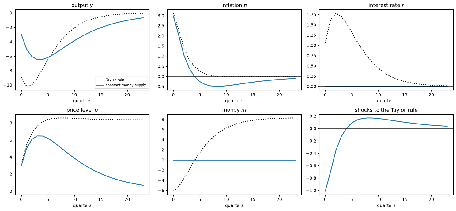
Fig. 32.3 A constant money supply#
money rule: max |r_t| = 2.5e-13, max |y_t + p_t| = 8.6e-14, y_0 = -2.98 (Taylor rule -8.95)
Under the money rule, inflation rises by less than under the Taylor rule and later undershoots, so that the price level returns to its initial value; under the Taylor rule, the price level rises permanently.
Output falls one for one with the price level, by 2.98 on impact against 8.95 under the Taylor rule; as under the fiscal-dominance peg, the recession is shallower but more persistent, bottoming out at \(-6.5\) in quarter 3.
The shocks to the Taylor rule that implement the money rule are first expansionary and then contractionary.
Exercise 32.2 finds the money-rule equilibrium among the peg equilibria and studies \(\gamma \neq 1\).
32.6. Forward guidance with imperfect commitment#
Caravello et al. [2026] also show that McKay and Wolf’s sufficient statistics deliver counterfactuals in which the rule itself switches stochastically, as in Davig and Leeper [2007].
The construction, which Policy Regimes and the Lucas Critique applies to a reversible tax reform, writes the counterfactual on the tree of policy histories.
Following their illustration, we study forward guidance with imperfect commitment.
The central bank pegs the interest rate at zero at date 0 and promises to keep it there until date \(H = 10\), after which the Taylor rule returns.
At each date \(t = 1, \ldots, H-1\), it abandons the peg with probability \(\omega = 0.24\).
Caravello et al. [2026] describe this as a reduced-form stand-in for the tension between commitment and discretion stressed by Kydland and Prescott [1977]; here it serves as a laboratory for the tree construction.
The histories form a simple tree.
Let \(N_t\) be the node at which the peg is still in place at date \(t\); the exit occurs at date \(k\) with probability \((1-\omega)^{k-1} \omega\) for \(k < H\), and at \(H\) with probability \((1-\omega)^{H-1}\).
After the exit, the Taylor rule holds, so the shocks to it are zero.
Let \(a_\ell\) be the shock at node \(N_\ell\), so that at node \(N_s\) the expected shock at date \(\ell \ge s\) is \((1-\omega)^{\ell - s} a_\ell\).
News arrives at each node \(N_s\) and at each exit.
At \(N_0\) the news about \(\nu_\ell\) is \((1-\omega)^\ell a_\ell\); at \(N_s\), \(s \ge 1\), it is \(\omega (1-\omega)^{\ell - s} a_\ell\); and at an exit at date \(k\) it is \(-(1-\omega)^{\ell - k + 1} a_\ell\).
News cannot be predictable: \((1-\omega)\) times the news at \(N_k\) plus \(\omega\) times the news at the exit is zero.
As in Policy Regimes and the Lucas Critique, the outcome at a node is the baseline response plus the effects of all the news received along the history that leads to it.
Because the private sector’s equations do not change over time, news that arrives at date \(s\) has the effects of the corresponding column of \(\Theta_\nu\) delayed by \(s\) periods.
The unknowns are \(a_0, \ldots, a_{H-1}\), and the equations are the peg at the nodes \(N_0, \ldots, N_{H-1}\).
def delayed(Θ, s):
    "Responses to news that arrives at date s: rows and columns of Θ shifted by s."
    out = np.zeros_like(Θ)
    for b in range(Θ.shape[0] // T):
        out[b * T + s:(b + 1) * T, s:] = Θ[b * T:(b + 1) * T - s, :T - s]
    return out

def forward_guidance(H, ω):
    """
    Peg at date 0; the Taylor rule returns with probability ω at each date 1, ..., H-1,
    and for sure at date H.  Returns the expected paths, the paths conditional on each
    exit date k = 1, ..., H, and their probabilities.
    """
    stay = 1 - ω
    def news_N(s):
        "News at N_s about the shocks ν_ℓ, as a T x H matrix acting on (a_0, ..., a_(H-1))."
        news = np.zeros((T, H))
        for ℓ in range(s, H):
            news[ℓ, ℓ] = stay**ℓ if s == 0 else ω * stay**(ℓ - s)
        return news
    effects = np.array([delayed(Θ_ν, s) @ news_N(s) for s in range(H + 1)])
    before = np.cumsum(effects[:H], axis=0)      # news at N_0, ..., N_s
    X_N = before[-1]
    a = np.linalg.solve(X_N[2 * T:2 * T + H], -x_A[2 * T:2 * T + H])
    path_N = x_A + X_N @ a
    branches = []
    for k in range(1, H + 1):
        # news at the exit node is -(stay/ω) times the news at N_k: news has mean zero
        exit_path = x_A + (before[k - 1] - (stay / ω) * effects[k]) @ a
        for b in range(5):
            exit_path[b * T:b * T + k] = path_N[b * T:b * T + k]
        branches.append(exit_path)
    probs = np.array([stay**(k - 1) * ω for k in range(1, H)] + [stay**(H - 1)])
    return probs @ np.array(branches), branches, probs

H_fg, ω_fg = 10, 0.24
x_fg, branches, probs = forward_guidance(H_fg, ω_fg)
To check the answer, we solve the model directly.
After an exit at date \(k\), the economy follows the Taylor rule under perfect foresight, starting from \(r_{k-1} = 0\) and the remaining path of the cost-push shock.
Before the exit, the IS and Phillips curves hold at each node \(N_t\) with \(r_t = 0\) and with expectations that average the next node and the exit, and we solve them backward from date \(H - 1\).
def forward_guidance_model(H, ω):
    "Expected (y, π, r) from the model's equations."
    stay = 1 - ω
    after = {}
    for k in range(1, H + 1):
        f_k = np.zeros(5 * T)
        f_k[T:2 * T - k] = e[k:]
        after[k] = np.column_stack(split(M_inv @ f_k)[:3])     # dated from k
    z_N = np.zeros((H, 2))
    for t in range(H - 1, -1, -1):
        z_exit = after[t + 1][0, :2]
        Ez = z_exit if t == H - 1 else stay * z_N[t + 1] + ω * z_exit
        y_t = Ez[0] + Ez[1] / γ
        z_N[t] = y_t, κ * y_t + β * Ez[1] + e[t]
    probs = np.array([stay**(k - 1) * ω for k in range(1, H)] + [stay**(H - 1)])
    out = np.zeros((80, 3))
    for k, pk in zip(range(1, H + 1), probs):
        for t in range(80):
            out[t] += pk * (np.append(z_N[t], 0.0) if t < k else after[k][t - k])
    return out

z_fg = forward_guidance_model(H_fg, ω_fg)
print(f"max |tree - model| over 60 quarters = "
      f"{np.abs(np.column_stack(split(x_fg)[:3])[:60] - z_fg[:60]).max():.1e}")
print(f"expected exit date {np.arange(1, H_fg + 1) @ probs:.1f}; "
      f"probability that the peg lasts until date H = {probs[-1]:.3f}")
max |tree - model| over 60 quarters = 1.9e-13
expected exit date 3.9; probability that the peg lasts until date H = 0.085
The tree construction reproduces the model’s answer to machine precision.
The peg is expected to end after about four quarters, and it lasts the full ten with probability 0.085.
We compare it with perfect commitment to the peg through date \(H - 1\).
ν_peg_H = np.linalg.solve(Θ_r[:H_fg, :H_fg], -x_A[2 * T:2 * T + H_fg])
x_peg_H = x_A + Θ_ν[:, :H_fg] @ ν_peg_H

fig, axes = plt.subplots(1, 3, figsize=(14, 4))
for i in range(3):
    for k in [1, 3, 6, H_fg]:
        axes[i].plot(split(branches[k - 1])[i][:H_plot], 'C0', lw=0.8, alpha=0.5)
    axes[i].plot(split(x_A)[i][:H_plot], 'k:', lw=2, label="Taylor rule")
    axes[i].plot(split(x_peg_H)[i][:H_plot], 'C4--', lw=2, label="perfect commitment")
    axes[i].plot(split(x_fg)[i][:H_plot], 'C0', lw=2.5, label="random exit, expected")
    axes[i].axhline(0, color='k', lw=0.5)
    axes[i].set_title(names[i])
    axes[i].set_xlabel("quarters")
axes[0].legend(fontsize=8)
plt.tight_layout()
plt.show()

for label, x in [("Taylor rule", x_A), ("perfect commitment", x_peg_H),
                 ("random exit", x_fg)]:
    print(f"{label:19s}: y_0 = {split(x)[0][0]:6.2f},  π_0 = {split(x)[1][0]:5.2f}")
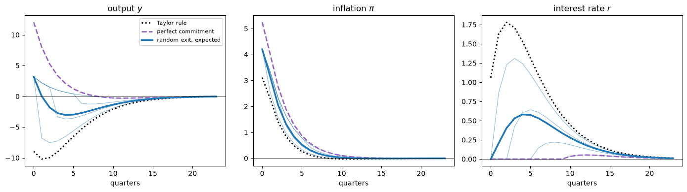
Fig. 32.4 Forward guidance with perfect and imperfect commitment#
Taylor rule        : y_0 =  -8.95,  π_0 =  3.11
perfect commitment : y_0 =  12.03,  π_0 =  5.24
random exit        : y_0 =   3.17,  π_0 =  4.20
The thin lines are the paths conditional on exits at dates 1, 3, 6, and 10.
A credible promise to hold the interest rate at zero for ten quarters turns the recession that the Taylor rule produces into a large boom and raises inflation on impact by two thirds.
Measured against the Taylor rule, imperfect commitment removes about 40 percent of the extra output on impact (output is 12.1 above its Taylor-rule value instead of 21.0) and about half of the extra inflation (1.09 instead of 2.13), because agents expect the Taylor rule to return early.
The size of the effect of a credible promise reflects the strength of forward guidance in this model, which is a property of the far-ahead columns of \(\Theta_\nu\).
Caravello et al. [2026] argue that the available evidence on monetary policy shocks speaks mainly to transitory changes in the interest rate, so that a counterfactual like this one depends on how a model extrapolates from those changes to the effects of distant ones.
32.7. Commitment and discretion#
Hebden and Winkler [2026] show that \(x_A\) and \(\Theta_\nu\) also suffice to compute optimal policy, both under commitment and under discretion.
We take the loss function \(\frac12 \sum_t \beta^t (\pi_t^2 + \lambda y_t^2)\) with \(\lambda = 0.1\), and collect its weights on the stacked paths in a diagonal matrix \(W_\lambda\).
Under commitment, the central bank chooses the whole path of rule shocks at date 0, a weighted least-squares problem, as in Exercise 29.1 of Policy Counterfactuals from Impulse Responses.
Under discretion, a sequence of policymakers each chooses the current interest rate and takes as given the rules that its successors follow.
Each policymaker sets policy so that \(d\, x^{(h)} = 0\), where \(x^{(h)}\) is the path expected at date \(h\), and we compute the row vector \(d\) with the algorithm of Exercise 29.3: given \(d\), the policymaker at date \(h\) chooses revisions \(\hat\nu\) of the rule shocks subject to her successors’ rules \(d\, F^k x^{(h)} = 0\), \(k \ge 1\), where \(F\) shifts a path forward one period, and her first-order condition delivers a new \(d\).
The result is a Markov perfect equilibrium, in the sense of the Markov perfect governments of Time Inconsistency of Ramsey Plans.
def loss_weights(λ):
    "The diagonal of W_λ: weights on the stacked paths of (y, π, r, p, m)."
    return np.concatenate([λ * disc, disc, np.zeros(3 * T)])

def commitment(λ):
    "Optimal plan under commitment: weighted least squares in the rule shocks."
    sqrt_w = np.sqrt(loss_weights(λ))
    ν_c, *_ = np.linalg.lstsq(sqrt_w[:, None] * Θ_ν, -sqrt_w * x_A, rcond=None)
    return x_A + Θ_ν @ ν_c

def stack_rules(d):
    "Rows d F^k, k = 0, ..., T-1, where F shifts each path forward one period."
    D = np.zeros((T, 5 * T))
    D[0] = d
    for k in range(1, T):
        for b in range(5):
            D[k, b * T + 1:(b + 1) * T] = D[k - 1, b * T:(b + 1) * T - 1]
    return D

def discretion(λ, tol=1e-14, max_iter=100):
    "The discretionary path, the Hebden–Winkler rule d, and the number of updates."
    w_λ = loss_weights(λ)
    Θ_0, Θ_rest = Θ_ν[:, 0], Θ_ν[:, 1:]
    d = Θ_0 * w_λ
    for it in range(max_iter):
        D_future = stack_rules(d)[1:]
        d_new = (Θ_0 - Θ_rest @ np.linalg.solve(D_future @ Θ_rest, D_future @ Θ_0)) * w_λ
        converged = np.abs(d_new - d).max() < tol
        d = d_new
        if converged:
            break
    D = stack_rules(d)
    return x_A + Θ_ν @ np.linalg.solve(D @ Θ_ν, -D @ x_A), d, it

λ = 0.1
w = loss_weights(λ)
x_comm = commitment(λ)
x_disc, d, it = discretion(λ)

y_c, π_c, _, p_c, _ = split(x_comm)
y_d, π_d, _, p_d, _ = split(x_disc)
y_c_lag = np.concatenate([[0.0], y_c[:-1]])
print(f"discretion: d stops changing after {it} update")
print(f"commitment: max |κ π_t + λ (y_t - y_(t-1))| = {np.abs(κ * π_c + λ * (y_c - y_c_lag))[:100].max():.1e}")
print(f"commitment: max |κ p_t + λ y_t|             = {np.abs(κ * p_c + λ * y_c)[:100].max():.1e}")
print(f"discretion: max |κ π_t + λ y_t|             = {np.abs(κ * π_d + λ * y_d)[:100].max():.1e}")
print(f"price level after 100 quarters: commitment {p_c[100]:.2f}, discretion {p_d[100]:.2f}")
loss = lambda x: 0.5 * np.sum(w * x**2)
print(f"loss: Taylor rule {loss(x_A):.2f}, commitment {loss(x_comm):.2f}, discretion {loss(x_disc):.2f}")
discretion: d stops changing after 1 update
commitment: max |κ π_t + λ (y_t - y_(t-1))| = 1.2e-13
commitment: max |κ p_t + λ y_t|             = 1.2e-13
discretion: max |κ π_t + λ y_t|             = 4.3e-14
price level after 100 quarters: commitment 0.03, discretion 16.56
loss: Taylor rule 36.02, commitment 16.91, discretion 23.16
The sequence-space calculations reproduce the familiar targeting rules: \(\kappa \pi_t + \lambda y_t = 0\) under discretion and \(\kappa \pi_t + \lambda (y_t - y_{t-1}) = 0\) under commitment [Clarida et al., 1999, Woodford, 2003].
Because the economy starts in the steady state, with \(y_{-1} = 0\), the date-0 Ramsey plan coincides here with the plan from the timeless perspective, which imposes the commitment targeting rule from date 0 on; a policymaker who re-optimized at a later date \(h\) would instead set \(\kappa \pi_h + \lambda y_h = 0\), ignoring \(y_{h-1}\), which is the time inconsistency discussed below.
Summing the commitment targeting rule from date 0 gives \(\kappa p_t + \lambda y_t = 0\): optimal policy under commitment is price-level targeting, and the price level returns to its initial value, while under discretion it rises permanently.
The first update of \(d\) is already the fixed point: the second update changes nothing.
Given her successors’ rules, a discretionary policymaker can affect only current output and inflation, because the private sector’s equations have no state variable through which today’s interest rate could affect the future (the price level is a state variable, but nothing depends on it).
That holds even though \(\Theta_\nu\) is not upper triangular here, as it is in the example of Hebden and Winkler [2026], because our baseline rule smooths the interest rate.
In the market of Policy Counterfactuals from Impulse Responses, where past quantities \(q_{t-1}, \ldots, q_{t-4}\) are state variables, the algorithm takes several updates.
fig, axes = plt.subplots(1, 3, figsize=(14, 4))
for x, style, label in [(x_A, 'k:', "Taylor rule"), (x_comm, 'C0', "commitment"),
                        (x_disc, 'C3--', "discretion")]:
    for i in range(3):
        axes[i].plot(split(x)[i][:H_plot], style, lw=2, label=label)
for i in range(3):
    axes[i].axhline(0, color='k', lw=0.5)
    axes[i].set_title(names[i])
    axes[i].set_xlabel("quarters")
axes[0].legend(fontsize=8)
plt.tight_layout()
plt.show()
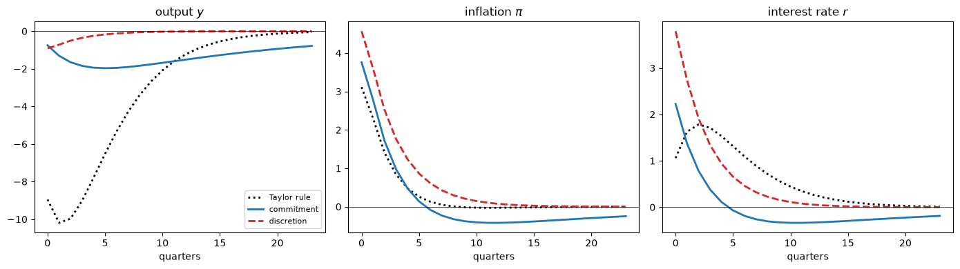
Fig. 32.5 Optimal policy under commitment and discretion#
Under commitment, the central bank promises to keep output below normal for longer, which lowers expected inflation and therefore current inflation, and it pulls the price level back; the discretionary policymaker cannot make that promise credibly, and its loss is higher.
As in Time Inconsistency of Ramsey Plans and Policy Counterfactuals from Impulse Responses, the commitment plan is time inconsistent, while the discretionary equilibrium is time consistent by construction.
32.8. Comparing the counterfactuals#
The loss function of the previous section ranks all the counterfactuals in this lecture.
For forward guidance with random exit we compute the expected loss across the branches of the tree, which exceeds the loss of the expected path.
w_π = np.concatenate([np.zeros(T), disc, np.zeros(3 * T)])       # the inflation part of W_λ
loss_π = lambda x: 0.5 * np.sum(w_π * x**2)
expected = lambda f: probs @ np.array([f(b) for b in branches])  # expectation across the tree
table = [("Taylor rule", loss(x_A), loss_π(x_A)),
         ("peg, monetary dominance", loss(x_md), loss_π(x_md)),
         ("peg, fiscal dominance", loss(x_fd), loss_π(x_fd)),
         ("constant money supply", loss(x_m), loss_π(x_m)),
         ("forward guidance, perfect commitment", loss(x_peg_H), loss_π(x_peg_H)),
         ("forward guidance, random exit (expected loss)", expected(loss), expected(loss_π)),
         ("optimal policy, discretion", loss(x_disc), loss_π(x_disc)),
         ("optimal policy, commitment", loss(x_comm), loss_π(x_comm))]
print(f"{'':48s}  {'loss':>6s}  {'inflation part':>14s}  {'output part':>11s}")
for label, total, part_π in sorted(table, key=lambda row: row[1]):
    print(f"{label:48s}  {total:6.1f}  {part_π:14.1f}  {total - part_π:11.1f}")
print(f"loss of the expected path under random exit: {loss(x_fg):.1f}")
                                                    loss  inflation part  output part
optimal policy, commitment                          16.9            14.2          2.7
optimal policy, discretion                          23.2            23.1          0.1
forward guidance, random exit (expected loss)       23.7            17.5          6.3
constant money supply                               26.0             8.2         17.9
peg, fiscal dominance                               26.5             8.0         18.5
Taylor rule                                         36.0             9.0         27.0
forward guidance, perfect commitment                41.5            28.8         12.7
peg, monetary dominance                             54.0            33.8         20.2
loss of the expected path under random exit: 20.4
Commitment does best, by construction.
Every policy that beats the Taylor rule does so by cutting the output part of the loss.
With a flat Phillips curve (\(\kappa = 0.02\)), lowering inflation costs a great deal of output, and \(\lambda = 0.1\) gives output enough weight that the Taylor rule’s recession is expensive.
Discretion goes furthest: it keeps output almost at its steady state and lets inflation run, so that its inflation part is about 2.6 times the Taylor rule’s.
The constant money supply and the peg under fiscal dominance, which with \(\gamma = 1\) are two members of the family of equilibria under the peg, keep the inflation part of the loss close to the Taylor rule’s (8.2 and 8.0 against 9.0) and produce recessions that are shallower but more persistent, with output parts about a third smaller than the Taylor rule’s.
Credible forward guidance and the monetary-dominance peg do worse than the Taylor rule because they let inflation run after a cost-push shock: their inflation parts are three to four times the Taylor rule’s.
The ranking depends on the loss.
The weight on output that a second-order approximation to household welfare implies in this model is \(\kappa / \varepsilon\), where \(\varepsilon\) is the elasticity of substitution among goods [Galí, 2015, Woodford, 2003].
With \(\varepsilon = 6\), as in Galí [2015], that weight is about 0.003, thirty times smaller than 0.1, and inflation matters much more.
The next cell ranks the counterfactuals again with that weight, recomputing the optimal policies under commitment and discretion for it; the other policies do not depend on the loss.
ε = 6                                    # elasticity of substitution among goods
λ_w = κ / ε
w_w = loss_weights(λ_w)
loss_w = lambda x: 0.5 * np.sum(w_w * x**2)
table_w = [("Taylor rule", loss_w(x_A)),
           ("peg, monetary dominance", loss_w(x_md)),
           ("peg, fiscal dominance", loss_w(x_fd)),
           ("constant money supply", loss_w(x_m)),
           ("forward guidance, perfect commitment", loss_w(x_peg_H)),
           ("forward guidance, random exit (expected loss)", expected(loss_w)),
           ("optimal policy, discretion", loss_w(discretion(λ_w)[0])),
           ("optimal policy, commitment", loss_w(commitment(λ_w)))]
print(f"welfare-based weight on output: κ / ε = {λ_w:.4f}")
for label, total in sorted(table_w, key=lambda row: row[1]):
    print(f"{label:48s}  {total:6.1f}")
welfare-based weight on output: κ / ε = 0.0033
optimal policy, commitment                           5.6
peg, fiscal dominance                                8.7
constant money supply                                8.8
Taylor rule                                          9.9
optimal policy, discretion                          13.2
forward guidance, random exit (expected loss)       17.7
forward guidance, perfect commitment                29.2
peg, monetary dominance                             34.4
With the welfare-based weight, commitment still does best, with a loss a little more than half the Taylor rule’s, and the peg under fiscal dominance and the constant money supply come next.
Discretion now does worse than the Taylor rule.
To hold down inflation, a discretionary policymaker can use only current output, and with a flat Phillips curve it engineers a recession twice as deep on impact as the Taylor rule’s yet is left with a larger inflation part of the loss.
The Taylor rule smooths the interest rate, so it keeps the rate high after the shock has faded, and the expectation of those high rates holds current inflation down: an inertial rule supplies some of the history dependence that commitment would, which is the stabilization bias of discretion seen from the other side [Woodford, 2003].
Forward guidance with random exit, third with \(\lambda = 0.1\), now falls behind the Taylor rule and discretion; credible forward guidance and the peg under monetary dominance remain far behind.
The ranking is for one shock and one loss function, and it says nothing about which of these policies a government could commit to.
32.9. What the extensions take for granted#
The extensions in this lecture keep the central assumption of McKay and Wolf [2023]: the private sector’s equations are linear and depend on policy only through the expected path of the instrument.
They add several assumptions of their own.
The data reveal every equilibrium under a counterfactual rule but not which one would occur, so the analyst must assume a criterion for equilibrium selection.
Fiscal policy matters here only through equilibrium selection because households are Ricardian; with non-Ricardian households, the timing of taxes matters, and the analyst also needs the causal effects of tax paths [Caravello et al., 2026].
A stochastic counterfactual, such as forward guidance with random exit, is still announced at date 0 and believed: it applies Lucas’s experiment to a process for rules rather than to a single rule, as Policy Regimes and the Lucas Critique discusses.
The discretionary equilibrium is one Markov perfect equilibrium, in which each policymaker follows a time-invariant linear rule; the theory of sustainable plans in Sustainable Plans for a Calvo Model admits others.
The econometrician here knows \(\Theta_\nu\) exactly, including the effects of news about distant dates; in practice, those effects must be extrapolated from evidence on a few policy shocks, as in the sections on limited evidence and on fitted models in Policy Counterfactuals from Impulse Responses.
32.10. Exercises#
Exercise 32.1
Sims [2011] argued that, under fiscal dominance, raising the interest rate to fight inflation can raise inflation instead, like stepping on a rake.
Compute the response to the cost-push shock under the more aggressive Taylor rule \(\phi_\pi = 3\) under monetary dominance, using McKay and Wolf’s construction.
Compute outcomes for the same path of the interest rate under fiscal dominance, using (32.6).
Compare inflation with that under the peg with fiscal dominance.
Solution
Under monetary dominance, the more aggressive rule is a rule like any other.
Under fiscal dominance, we cannot simply impose the rule, because with an active Taylor rule and an active fiscal policy there is generically no bounded equilibrium.
Instead we fix the path of the interest rate that the \(\phi_\pi = 3\) rule produces under monetary dominance
and use peg_equilibria with that path as the target, as Caravello et al. [2026] do in their
application to U.S. inflation after 2021.
R_3 = taylor_rule(3.0)
ν_3 = np.linalg.solve(R_3 @ Θ_ν, -R_3 @ x_A)
x_3 = x_A + Θ_ν @ ν_3
r_3 = split(x_3)[2]
x_3_md, _, x_3_fd, _ = peg_equilibria(r_3[:K])

fig, axes = plt.subplots(1, 2, figsize=(12, 4))
for x, style, label in [(x_A, 'k:', "Taylor rule, $\\phi_\\pi = 1.7$"),
                        (x_3_md, 'C0', "$\\phi_\\pi = 3$ rate path, monetary dominance"),
                        (x_3_fd, 'C3', "$\\phi_\\pi = 3$ rate path, fiscal dominance"),
                        (x_fd, 'C1--', "peg, fiscal dominance")]:
    for j, i in enumerate([1, 2]):
        axes[j].plot(split(x)[i][:H_plot], style, lw=2, label=label)
for j, i in enumerate([1, 2]):
    axes[j].axhline(0, color='k', lw=0.5)
    axes[j].set_title(names[i])
    axes[j].set_xlabel("quarters")
axes[0].legend(fontsize=8)
plt.tight_layout()
plt.show()

print(f"π_0: φ_π = 3 under monetary dominance {split(x_3_md)[1][0]:.2f}, same rates under fiscal "
      f"dominance {split(x_3_fd)[1][0]:.2f}, peg under fiscal dominance {split(x_fd)[1][0]:.2f}")
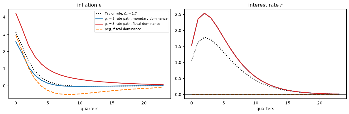
π_0: φ_π = 3 under monetary dominance 2.56, same rates under fiscal dominance 4.22, peg under fiscal dominance 2.95
Under monetary dominance, the aggressive rule lowers inflation, as intended.
Under fiscal dominance, the same path of higher interest rates raises inflation relative to the peg.
By (32.6), higher interest payments on the debt, unbacked by taxes, must be paid for by higher discounted inflation.
With the one-period debt of this model, inflation rises at once; in Sims [2011], long-term debt makes a higher interest rate lower inflation at first and raise it later.
Exercise 32.2
The main text showed that, with \(\gamma = 1\), a constant money supply keeps the interest rate at zero, so that its equilibrium is one of the equilibria under the peg.
Find that member of the family of peg equilibria with McKay and Wolf’s objects, using the fact that the price level returns to its initial value, and compare it with the money-rule equilibrium.
Compare it with the fiscal-dominance equilibrium.
Repeat the money-rule calculation with \(\gamma = 2\), and show that the interest rate now moves but the price level still returns to its initial value.
Solution
The price level returns to its initial value when undiscounted cumulative inflation is zero, so we add to the monetary-dominance equilibrium the multiple of the sunspot direction that sets \(\sum_t \pi_t = 0\).
c_m = -split(x_md)[1].sum() / π_h.sum()
x_sum0 = x_md + c_m * x_h
print(f"max |peg equilibrium with Σ π_t = 0 - money rule| over 60 quarters = "
      f"{np.abs(split(x_sum0)[1][:60] - split(x_m)[1][:60]).max():.1e}")
print(f"π_0: money rule {split(x_m)[1][0]:.3f}, fiscal dominance {split(x_fd)[1][0]:.3f}")

M_inv_2 = np.linalg.inv(np.vstack([private_block(γ=2.0), taylor_rule()]))
x_A_2, Θ_2 = M_inv_2 @ forcing(), M_inv_2[:, 4 * T:]
x_m_2 = x_A_2 + Θ_2 @ np.linalg.solve(R_m @ Θ_2, -R_m @ x_A_2)
print(f"γ = 2: interest rate under the money rule, first quarters: {np.round(split(x_m_2)[2][:4], 3)}")
print(f"γ = 2: price level after 100 quarters: {split(x_m_2)[3][100]:.1e}")
max |peg equilibrium with Σ π_t = 0 - money rule| over 60 quarters = 1.8e-07
π_0: money rule 2.978, fiscal dominance 2.951
γ = 2: interest rate under the money rule, first quarters: [-1.557 -0.739 -0.212  0.118]
γ = 2: price level after 100 quarters: 1.8e-05
With \(\gamma = 1\), the money rule picks the peg equilibrium in which undiscounted cumulative inflation is zero; the fiscal theory picks the one in which discounted cumulative inflation is zero, which is close to it because \(\beta\) is close to one.
With \(\gamma = 2\), the right side of the equation for \(r_t\) in the main text is no longer zero, so the interest rate moves under the money rule; the price level still returns to its initial value, because \(p_t = \eta r_t - y_t\) and both \(r_t\) and \(y_t\) return to zero.
Exercise 32.3
The forward guidance puzzle [Del Negro et al., 2023] is that, in models like this one, promises about distant interest rates have very large effects today.
For promised durations \(H = 2, 4, \ldots, 16\) of the peg, compute the impact responses of output and inflation under perfect commitment and under exit probabilities \(\omega = 0.1\) and \(\omega = 0.24\), and compare them with the peg that lasts forever under monetary dominance.
Starting from the steady state, compute the impact responses of output and inflation to a promise to cut the interest rate by one point at date \(\ell\) only, for \(\ell = 0, 8, 20, 40\), under monetary dominance and under fiscal dominance.
Solution
Hs = np.arange(2, 17, 2)
fig, axes = plt.subplots(1, 2, figsize=(12, 4))
for ω_i, style in [(None, 'C4--'), (0.1, 'C0-o'), (0.24, 'C2-s')]:
    impact = []
    for H_i in Hs:
        if ω_i is None:
            ν_i = np.linalg.solve(Θ_r[:H_i, :H_i], -x_A[2 * T:2 * T + H_i])
            x_i = x_A + Θ_ν[:, :H_i] @ ν_i
        else:
            x_i, _, _ = forward_guidance(H_i, ω_i)
        impact.append([split(x_i)[0][0], split(x_i)[1][0]])
    impact = np.array(impact)
    label = "perfect commitment" if ω_i is None else f"exit probability {ω_i}"
    for j in range(2):
        axes[j].plot(Hs, impact[:, j], style, lw=2, label=label)
for j in range(2):
    axes[j].axhline(split(x_md)[j][0], color='C4', lw=1, ls=':', label="peg forever, monetary dominance")
    axes[j].set_title(f"impact response of {names[j]}")
    axes[j].set_xlabel("promised duration of the peg $H$ (quarters)")
axes[0].legend(fontsize=8)
plt.tight_layout()
plt.show()
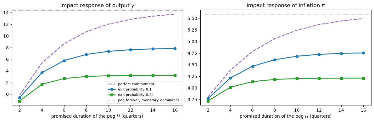
Under perfect commitment, the impact effect on output rises quickly with the promised duration, from \(-0.2\) at \(H = 2\) to \(12.0\) at \(H = 10\), and then approaches the effect of the peg that lasts forever under monetary dominance, \(14.4\), which it nearly reaches by \(H = 30\) (not shown).
The effects level off because the peg replaces the Taylor rule’s response to a cost-push shock that dies out: once the peg outlasts most of the shock, lengthening it changes little.
With random exit, they level off sooner and at much lower values: a promise that is likely to be abandoned before it matters has little effect.
The second part isolates the puzzle: a cut at a single date, from the steady state, with no shock to respond to.
zero = np.zeros(5 * T)
print("  ℓ   monetary dominance: y_0      π_0     fiscal dominance: y_0      π_0")
for ℓ in [0, 8, 20, 40]:
    cut = np.zeros(K)
    cut[ℓ] = -1.0
    x_cut_md, _, x_cut_fd, _ = peg_equilibria(cut, x_base=zero)
    print(f"{ℓ:3d}   {split(x_cut_md)[0][0]:22.3f} {split(x_cut_md)[1][0]:8.3f}   "
          f"{split(x_cut_fd)[0][0]:20.4f} {split(x_cut_fd)[1][0]:8.4f}")
print(f"1 / μ_s = {1 / μ_s:.3f}")
  ℓ   monetary dominance: y_0      π_0     fiscal dominance: y_0      π_0
  0                    1.000    0.020                 0.1008  -0.1153
  8                    1.803    0.230                 0.0322  -0.0368
 20                    8.927    1.335                 0.0058  -0.0066
 40                  146.784   22.081                 0.0003  -0.0004
1 / μ_s = 1.150
Under monetary dominance, the effect today of a cut at date \(\ell\) grows with \(\ell\), eventually by the factor \(1 / \mu_s \approx 1.15\) per quarter of delay: that is the forward guidance puzzle.
This version of the experiment cuts the nominal rate at date \(\ell\) and holds it at its steady-state value at all other dates, so that before date \(\ell\) the economy follows the pegged system solved backward from date \(\ell\); solving it backward multiplies by the inverse of its stable root, \(1 / \mu_s\), each quarter.
In the experiment of McKay et al. [2016], which cuts the real rate at date \(\ell\) and holds it at its steady-state value at all other dates, the effect on output today does not depend on \(\ell\), while the effect on inflation grows with \(\ell\) toward a bound, \(\kappa / (\gamma (1 - \beta)) \approx 8\), rather than without limit.
Under fiscal dominance, the same promise barely moves output and lowers inflation, because, by (32.6), lower interest payments on the debt must be matched by lower discounted inflation; Cochrane [2023] argues that the fiscal theory removes the puzzle in this way.
Imperfect credibility, as in the first part, is another proposed resolution, and weaker responses to distant news, as in the cognitive discounting of Gabaix [2020], are a third.
Caravello et al. [2026] find that, with rational expectations, perfect and stochastic commitment to forward guidance give very different counterfactuals, while with cognitive discounting they give similar ones, so the choice of model for extrapolating \(\Theta_\nu\) matters for questions like this one.