
30. Invertibility and Policy Counterfactuals#
30.1. Overview#
Policy Counterfactuals from Impulse Responses adds a tax to the market of Dynamic Supply and Demand Curves and shows that, as McKay and Wolf [2023] prove in general, impulse responses to a non-policy shock and to contemporaneous and news shocks to the tax rule deliver the market’s behavior under a different rule.
That lecture takes those impulse responses as known.
This lecture asks what it takes to estimate them, a question that connects McKay and Wolf’s method to the theme of Dynamic Supply and Demand Curves and Induced Priors for Impulse Responses, in which the supply shock is not fundamental for prices and quantities.
In this market,
a local projection on an instrument recovers the supply-shock impulse response that no rotation of VAR innovations can, while the “external instrument” method, which uses the instrument to select such a rotation, does not, although in samples of realistic length the local projection is noisy,
whether the supply shock is fundamental depends on the policy rule — a version of the Lucas critique that applies to VAR identification itself — because a price-stabilizing tax rule is observationally equivalent to making suppliers more flexible, and
McKay and Wolf’s route to counterfactual second moments through VAR innovations is exact under invertibility, and in this market the error it makes otherwise turns out to be tiny: supply shocks account for less than half a percent of the variance of prices and quantities, so forecasts based on prices and quantities are almost as good as forecasts based on the shocks themselves.
In addition to what’s in Anaconda, this lecture uses the quantecon library.
!pip install --upgrade quantecon
We’ll make these imports:
import numpy as np
import quantecon as qe
import matplotlib.pyplot as plt
30.2. The market with a tax#
We use the market of Policy Counterfactuals from Impulse Responses, with the same parameters and the same code.
The supplier pays a tax \(\tau_t\) per unit, set by the rule \(\tau_t = -\phi p_t + \nu_t\), and we stack the supply and demand curves and the rule for \(t = 0, \ldots, T-1\) into one linear system.
h_s = h_d = 1.0
g_s, g_d = 10.0, 0.1
β = 1 / 1.05
a = np.array([1, .8, .6, .4, .2])       # a(L): coefficients a0..a4

# MA polynomials for the shocks (coefficients on L^0..L^3)
B_d = np.convolve(np.convolve([1, .6], [1, .4]), [1, .2])
B_s = np.convolve(np.convolve([1, -.8], [1, .4]), [1, .2])

σ_s, σ_d = np.sqrt(0.5), 2.0            # shock standard deviations
T = 200     # length of the stacked paths

def private_block(g_s, g_d, T=T, h_s=h_s):
    """
    Stack the Euler equations for t = 0, ..., T-1.

    Unknowns are ordered x = (q, p, τ), each a path of length T, and the
    equations read  H @ x = (s, -d).
    """
    Φ_s, Φ_d = np.zeros((T, T)), np.zeros((T, T))
    for t in range(T):
        Φ_s[t, t] += h_s + g_s * (1 + β)
        if t >= 1:
            Φ_s[t, t - 1] -= g_s
        if t + 1 < T:
            Φ_s[t, t + 1] -= g_s * β
        Φ_d[t, t] += h_d
        for i in range(5):
            for k in range(5):
                if 0 <= t + i - k < T:
                    Φ_d[t, t + i - k] += g_d * a[i] * a[k] * β**i
    I, O = np.eye(T), np.zeros((T, T))
    return np.block([[-Φ_s, I, -I],      # supply:  p - τ - Φ_s q = s
                     [Φ_d, I, O]])       # demand:  p + Φ_d q = -d

def rule_block(φ, T=T):
    "The rule τ = -φ p + ν written as  R @ x = ν."
    return np.hstack([np.zeros((T, T)), φ * np.eye(T), np.eye(T)])

def system_inverse(g_s, g_d, φ, h_s=h_s):
    "Inverse of the stacked system: x = inverse @ (s, -d, ν)."
    return np.linalg.inv(np.vstack([private_block(g_s, g_d, h_s=h_s), rule_block(φ)]))

def forcing(shock, T=T, σ_s=σ_s):
    "Right-hand side for a favorable supply shock (0) or a positive demand shock (1)."
    s, d = np.zeros(T), np.zeros(T)
    if shock == 0:
        s[:4] = -σ_s * B_s
    else:
        d[:4] = -σ_d * B_d
    return np.concatenate([s, -d, np.zeros(T)])

def split(x):
    "Split a stacked path into (q, p, τ)."
    return x[:T], x[T:2 * T], x[2 * T:]
The policy shock is \(\nu_t = \sum_{\ell \ge 0} \nu_{\ell, t-\ell}\), where \(\nu_{0,t}\) is a contemporaneous surprise and \(\nu_{\ell, t-\ell}\), \(\ell > 0\), is news, received at date \(t - \ell\), of a deviation from the rule at date \(t\).
Stack the paths of quantity, price, and the tax into \(x = (q, p, \tau)\) and write the rule as \(R\, x = \nu\).
Let \(x_A(\varepsilon)\) be the response to a non-policy shock \(\varepsilon\) under the baseline rule, and let \(\Theta_\nu\) be the matrix whose column \(\ell\) is the response to news, received at date 0, of a unit shock to the rule at date \(\ell\).
McKay and Wolf’s Proposition 1 says that, under a counterfactual rule \(\tilde R\, x = 0\), the response to \(\varepsilon\) is
The function below implements (30.1): it enforces a new rule with date-0 policy shocks.
def mw_counterfactual(M_inv_base, x_A, φ_new):
    "McKay–Wolf Proposition 1: enforce τ = -φ_new p with date-0 policy shocks."
    Θ = M_inv_base[:, 2 * T:]
    R_new = rule_block(φ_new)
    ν = np.linalg.solve(R_new @ Θ, -R_new @ x_A)
    return x_A + Θ @ ν, ν
As in Policy Counterfactuals from Impulse Responses, the baseline rule is \(\phi_A = 0.5\) and the counterfactual rule is \(\tilde\phi = 2\).
φ_A, φ_new = 0.5, 2.0
M_inv_A = system_inverse(g_s, g_d, φ_A)
H_plot = 20
names = ["quantity $q$", "price $p$", "tax $\\tau$"]
rng = np.random.default_rng(1234)
30.3. The supply shock is not fundamental#
Estimating \(x_A(\varepsilon)\) and \(\Theta_\nu\) requires identifying assumptions.
In Dynamic Supply and Demand Curves and Induced Priors for Impulse Responses we saw that, because quantity adjusts sluggishly, the supply shock is not fundamental for \((q_t, p_t)\): it is not a linear combination of current and past prices and quantities.
No rotation of the innovations of a vector autoregression for \((q_t, p_t)\) recovers the supply shock — not a Cholesky factorization, and not one selected by sign restrictions.
We work in what follows with the economy under the baseline rule and no policy shocks, so that the econometrician observes \((q_t, p_t)\) and \(\tau_t = -\phi_A p_t\).
That choice does three things.
The tax is then a fixed multiple of the price and adds no information, so the vector autoregression can be in \((q_t, p_t)\) alone.
The data have two shocks for two observables; with policy shocks, news included, there would be more shocks than observables.
And \(\Theta_\nu\) cannot be estimated from these data: we treat it as known, as if measured from instruments for the policy shocks, and focus on the non-policy shocks.
The cost and demand shocks are \(s_t = B_s(L) w_{st}\) and \(d_t = B_d(L) w_{dt}\), as in Dynamic Supply and Demand Curves, with \(w_{st}\) and \(w_{dt}\) independent with standard deviations \(\sigma_s\) and \(\sigma_d\).
As in Induced Priors for Impulse Responses, we work with a favorable supply shock \(\tilde w_{st} = -w_{st}\) and a positive demand shock \(\tilde w_{dt} = -w_{dt}\), both of which raise quantity.
Write the structural moving average as \(z_t = (q_t, p_t)^\top = \sum_{j \ge 0} D_j \epsilon_{t-j}\), where \(\epsilon_t = (\tilde w_{st} / \sigma_s, \tilde w_{dt} / \sigma_d)^\top\) stacks the two shocks scaled to unit variance, and the Wold representation as
where \(u_t = z_t - \mathbb{E}[z_t \mid z_{t-1}, z_{t-2}, \ldots]\) is the innovation of a vector autoregression of infinite order and \(L\) is the lower-triangular Cholesky factor of \(V\), as in Induced Priors for Impulse Responses; the lag operator appears only inside polynomials such as \(B_s(L)\).
The impact responses to the two shocks are the columns \(d_s\) and \(d_d\) of \(D_0\).
The demand shock is fundamental in this market to within \(10^{-6}\), as the code below shows, so the moving average is invertible exactly when the supply shock is fundamental, and we use the two terms interchangeably.
To compute the Wold representation, we write the moving-average representation, truncated after H_ma
lags, in state-space form, with the current and lagged shocks as the state, and apply the Kalman filter;
Dynamic Supply and Demand Curves applies the same filter to the market’s equilibrium state.
A First Look at the Kalman Filter introduces the filter, and Classical Prediction and Filtering With Linear Algebra derives the same Wold representation by factoring the spectral density.
H_ma = 80    # truncation lag for the moving-average representation

def structural_ma(g_s, g_d, φ, h_s=h_s, σ_s=σ_s):
    "Stacked responses of (q, p, τ) to the two structural shocks: a 3T x 2 array."
    M_inv = system_inverse(g_s, g_d, φ, h_s=h_s)
    return np.stack([M_inv @ forcing(k, σ_s=σ_s) for k in range(2)], axis=1)

def ma_qp(X):
    "MA coefficients D_j (2 x 2) of (q, p) from stacked paths, j = 0..H_ma-1."
    return np.stack([X[:H_ma], X[T:T + H_ma]], axis=1)

def wold(D):
    "Innovation covariance V and Wold MA coefficients C_j of z_t = sum_j D_j ε_(t-j)."
    k = D.shape[2]
    n = H_ma * k
    A = np.zeros((n, n)); A[k:, :-k] = np.eye(n - k)
    C = np.zeros((n, k)); C[:k] = np.eye(k)
    G = np.hstack(list(D))
    kalman = qe.Kalman(qe.LinearStateSpace(A, C, G, 1e-8 * np.eye(D.shape[1])))
    kalman.stationary_values()
    V = kalman.stationary_innovation_covar()
    C_wold = np.array(kalman.stationary_coefficients(H_ma - 1, 'ma'))
    return V, C_wold

def impulse_norms(D, V):
    "||L^{-1} d|| for each structural impact vector d (columns of D_0)."
    return np.linalg.norm(np.linalg.solve(np.linalg.cholesky(V), D[0]), axis=0)

X_A = structural_ma(g_s, g_d, φ_A)
D_A = ma_qp(X_A)
V_A, C_wold_A = wold(D_A)
norms_A = impulse_norms(D_A, V_A)
print(f"||L^-1 d|| under the baseline rule: supply {norms_A[0]:.4f}, demand {norms_A[1]:.7f}")
||L^-1 d|| under the baseline rule: supply 0.8662, demand 0.9999994
As in Induced Priors for Impulse Responses, a norm below one says that the supply impact vector is not a rotation of the VAR innovations.
The norm has a direct interpretation.
Because the supply shock is uncorrelated with past prices and quantities, its projection on current and past \(z\) is its projection on \(u_t\), and the \(R^2\) of that projection is \(d_s^\top V^{-1} d_s = \|L^{-1} d_s\|^2\).
Here \(\|L^{-1} d_s\|^2 = 0.866^2 = 0.75\): data through date \(t\) reveal three quarters of the variance of the date-\(t\) supply shock, and later data reveal the rest.
30.4. Local projections on an instrument do not need invertibility#
Write \(\epsilon_{st} = \tilde w_{st} / \sigma_s\) for the favorable supply shock scaled to unit variance.
Suppose that the econometrician observes a noisy measure of the supply shock — for example, a series on unanticipated changes in input costs —
where \(v_t\) is measurement error with unit variance, independent of everything else.
(A series on input costs themselves, \(s_t = B_s(L) w_{st}\), would also serve as long as the projections control for enough of its lags: because \(B_s\) has its zeros outside the unit circle, the innovation in \(s_t\) is the supply shock itself, and observing \(s_t\) would make the supply shock fundamental for \((q_t, p_t, s_t)\).)
Let \(D_h^{(s)}\) be the first column of \(D_h\), so that \(D_0^{(s)} = d_s\).
Because \(\epsilon_{st}\) is serially uncorrelated and independent of the demand shock,
the true response of \(z\) at horizon \(h\) to the supply shock.
A local projection of \(z_{t+h}\) on \(m_t\) therefore recovers the supply-shock impulse response up to scale, whether or not the supply shock is fundamental.
Dividing by the coefficient in the projection of \(q_t\) on \(m_t\) normalizes the response to raise quantity by one unit on impact; the ratio is the instrumental-variables estimate of a regression of \(z_{t+h}\) on \(q_t\) with instrument \(m_t\), the estimator known as LP-IV.
In samples, the projections also include lags of the data as controls, which improves precision without changing the population estimand.
Stock and Watson [2018] develop this logic, and Plagborg-Møller and Wolf [2021] show that ordering the instrument first in a recursive VAR, an “internal instrument” VAR, estimates the same impulse responses.
The terminology deserves care.
The method known in the literature as “external instruments”, SVAR-IV, or proxy SVAR, proposed by Stock [2008] and used by Mertens and Ravn [2013], uses the instrument only to select a rotation of the VAR innovations.
It sets the impact vector proportional to \(\mathrm{cov}(u_t, m_t)\) and lets the VAR’s moving-average coefficients propagate it.
That method needs invertibility.
In population, \(\mathrm{cov}(u_t, m_t) = \mathrm{cov}(z_t, \epsilon_{st}) = d_s\), because the supply shock is uncorrelated with past prices and quantities, so SVAR-IV gets the direction of the impact response right and gives \(C_h d_s\) at horizon \(h\).
SVAR-IV also gets the size of the impact response wrong when the shock is not fundamental.
Normalizing the identified shock to unit variance gives the impact response \(d_s / \|L^{-1} d_s\|\), which overstates the response to a one-standard-deviation supply shock by the factor \(1/0.866 \approx 1.15\); under invertibility the norm is one and SVAR-IV gets absolute responses right [Plagborg-Møller and Wolf, 2021].
McKay and Wolf estimate the responses to their non-policy shock with the invertibility-robust method: they order the series of investment-specific technology news shocks of Ben Zeev and Khan [2015] first in a VAR.
We simulate a long sample under the baseline rule and compare the true response to a supply shock with two estimates from the simulated sample and two population benchmarks, each normalized to raise quantity by one unit on impact:
a local projection on \(m_t\), with four lags of \((m_t, q_t, p_t)\) as controls,
a VAR in \((m_t, q_t, p_t)\) with 12 lags and \(m_t\) ordered first, the internal-instrument VAR,
SVAR-IV, computed from the population Wold representation, and
the second shock of a Cholesky factorization of the population VAR innovations, with the price ordered first.
The last is the shock that does not move the price on impact; Induced Priors for Impulse Responses shows that it is an edge of the set of supply shocks that the theory’s sign restrictions admit, and it misses the true impact response of price by construction.
n_sim = 2_000_000
ε = rng.standard_normal((n_sim + H_ma, 2))
m = ε[H_ma:, 0] + rng.standard_normal(n_sim)        # noisy proxy for the supply shock

# simulate (q, p) from the moving-average representation
x_sim = np.zeros((n_sim, 2))
for i in range(2):
    for k in range(2):
        x_sim[:, i] += np.convolve(ε[:, k], D_A[:, i, k])[H_ma:H_ma + n_sim]

def lagged(Y, p):
    "Columns Y_(t-1), ..., Y_(t-p) for t = p, ..., len(Y) - 1."
    return np.hstack([Y[p - j:len(Y) - j] for j in range(1, p + 1)])

def lp_iv(z, m, p, n_h):
    "LP-IV responses of z to the instrument m, with p lags of (m, z) as controls, unit impact on q."
    W = np.column_stack([m, z])
    controls = np.column_stack([np.ones(len(z) - p), lagged(W, p)])
    def residual(y, X):
        coef, *_ = np.linalg.lstsq(X, y, rcond=None)
        return y - X @ coef
    out = np.zeros((n_h, z.shape[1]))
    for h in range(n_h):
        X_h = controls[:len(z) - p - h]
        m_h = residual(m[p:len(z) - h], X_h)
        out[h] = [m_h @ residual(z[p + h:, i], X_h) / (m_h @ m_h) for i in range(z.shape[1])]
    return out / out[0, 0]

# local projections on the proxy, horizons 0, ..., 12
lp = lp_iv(x_sim, m, 4, 13)

def var_fit(Y, p):
    "Least-squares VAR(p) with a constant: coefficient matrices A_1..A_p and residuals."
    X = np.column_stack([np.ones(len(Y) - p), lagged(Y, p)])
    coef, *_ = np.linalg.lstsq(X, Y[p:], rcond=None)
    k = Y.shape[1]
    return [coef[1 + j * k:1 + (j + 1) * k].T for j in range(p)], Y[p:] - X @ coef

def var_ma(A_list, n_h):
    "Moving-average coefficients Ψ_0, ..., Ψ_(n_h - 1) of a VAR."
    Ψ = [np.eye(A_list[0].shape[0])]
    for h in range(1, n_h):
        Ψ.append(sum(A_list[j] @ Ψ[h - 1 - j] for j in range(min(len(A_list), h))))
    return np.array(Ψ)

# internal-instrument VAR: (m, q, p) with m ordered first
A_iv, U_iv = var_fit(np.column_stack([m, x_sim]), 12)
int_iv = var_ma(A_iv, H_plot) @ np.linalg.cholesky(np.cov(U_iv.T))[:, 0]
int_iv = int_iv[:, 1:] / int_iv[0, 1]

truth = D_A[:H_plot, :, 0] / D_A[0, 0, 0]

# the population VAR's p-first Cholesky factorization: the second shock has no impact on p
P_swap = np.array([[0, 1], [1, 0]])
L_p = P_swap @ np.linalg.cholesky(P_swap @ V_A @ P_swap)
chol = np.array([C_wold_A[h] @ L_p[:, 1] for h in range(H_plot)])
chol /= chol[0, 0]

# SVAR-IV: impact vector cov(u_t, m_t) = d_s, propagated by the Wold coefficients
svar_iv = np.array([C_wold_A[h] @ D_A[0][:, 0] for h in range(H_plot)])
svar_iv /= svar_iv[0, 0]

fig, axes = plt.subplots(1, 2, figsize=(12, 4))
for i, ax in enumerate(axes):
    ax.plot(truth[:, i], 'k-', lw=2, label="true supply-shock response")
    ax.plot(lp[:, i], 'C0o', ms=5, label="local projection on the proxy $m_t$")
    ax.plot(int_iv[:, i], 'C1x', ms=7, label="VAR with $m_t$ ordered first")
    ax.plot(svar_iv[:, i], 'C2-.', lw=2, label="SVAR-IV (external instrument), population")
    ax.plot(chol[:, i], 'C3--', lw=2, label="VAR, p-first Cholesky, population")
    ax.axhline(0, color='k', lw=0.5)
    ax.set_title(f"response of {names[i]} (unit impact on $q$)")
    ax.set_xlabel("periods")
    ax.set_xlim(0, 12)
axes[0].legend(fontsize=8)
plt.tight_layout()
plt.show()
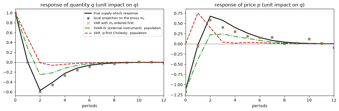
Fig. 30.1 Recovering the supply-shock response#
The local projection recovers the true response, including the sign reversal after two periods, while the Cholesky-identified VAR shock does not.
Even in 2,000,000 periods, sampling error remains visible, especially for the price, because supply shocks account for so little of the variation in the data.
The internal-instrument VAR delivers nearly the same estimates as the local projection.
Plagborg-Møller and Wolf [2021] prove that, in population, a VAR with \(p\) lags and a local projection that controls for \(p\) lags estimate the same impulse responses out to horizon \(p\).
Here the VAR has 12 lags and the projection controls for 4, but the conclusion carries over: because \(m_t\) is unpredictable from the past, the projection’s estimand does not depend on how many lags it controls for, so both recover the true response out to horizon 12.
SVAR-IV gets the direction of the impact response right, but it propagates the impact vector with the VAR’s moving-average coefficients, which do not describe how a non-fundamental shock propagates: it overstates the responses one period after the shock and shows only a third to a half of the reversal that follows.
This is the constructive counterpart of the negative results in Induced Priors for Impulse Responses: information from outside the VAR — here, a measured cost shock — can recover a shock that prices and quantities alone reveal only with a delay.
McKay and Wolf’s conditional counterfactuals in Proposition 1 have the same property as the local projection: they need impulse responses to the non-policy shock and to the policy shocks, and if those are estimated by projections on instruments, invertibility plays no role.
In McKay and Wolf’s applications the responses to policy shocks come from instruments, such as narrative measures or high-frequency financial market surprises.
Anticipated policy shocks are themselves a standard source of non-invertibility — see Leeper et al. [2013] on fiscal foresight, and Shock Non Invertibility for the same “news” problem in a permanent income model — which is another reason why McKay and Wolf identify policy shocks with instruments.
30.4.1. Samples of realistic length#
We used a very long sample because supply shocks account for only a small part of the variation in prices and quantities.
The next figure repeats the comparison in 400 samples of 200 periods, with twelve lags as controls in each estimator, for the baseline shock sizes and for a supply shock whose standard deviation is \(\sigma_s = 4\).
It plots the median estimate of the response of quantity and the range between the 25th and 75th percentiles.
def estimates(z, m, p=12, n_h=9):
    "LP-IV, internal-instrument VAR, and SVAR-IV responses of (q, p), normalized to a unit impact on q."
    lp_est = lp_iv(z, m, p, n_h)
    W = np.column_stack([m, z])
    A_w, U_w = var_fit(W, p)
    iv_est = var_ma(A_w, n_h) @ np.linalg.cholesky(np.cov(U_w.T))[:, 0]
    A_z, U_z = var_fit(z, p)
    sv_est = var_ma(A_z, n_h) @ (U_z.T @ m[p:] / len(U_z))
    return [lp_est] + [e / e[0, 0] for e in (iv_est[:, 1:], sv_est)]

def simulate_sample(D, n, rng):
    "Simulate (q, p) from the moving average D and a noisy proxy for the supply shock."
    ε_s = rng.standard_normal((n + H_ma, 2))
    m_s = ε_s[H_ma:, 0] + rng.standard_normal(n)
    z_s = np.zeros((n, 2))
    for i in range(2):
        for k in range(2):
            z_s[:, i] += np.convolve(ε_s[:, k], D[:, i, k])[H_ma:H_ma + n]
    return z_s, m_s

n_rep, n_obs, n_h = 400, 200, 9
fig, axes = plt.subplots(1, 2, figsize=(12, 4), sharey=True)
for ax, σ in zip(axes, [σ_s, 4.0]):
    D_σ = ma_qp(structural_ma(g_s, g_d, φ_A, σ_s=σ))
    draws = np.array([estimates(*simulate_sample(D_σ, n_obs, rng))
                      for _ in range(n_rep)])[:, :, :, 0]      # replication, method, horizon
    ax.plot(D_σ[:n_h, 0, 0] / D_σ[0, 0, 0], 'k-', lw=2, label="true response")
    C_σ = wold(D_σ)[1]
    sv_pop = np.array([C_σ[h] @ D_σ[0][:, 0] for h in range(n_h)])
    ax.plot(sv_pop[:, 0] / sv_pop[0, 0], 'C2--', lw=1.5, label="SVAR-IV, population")
    for j, (label, color) in enumerate([("LP-IV", 'C0'), ("VAR with $m_t$ first", 'C1'),
                                        ("SVAR-IV", 'C2')]):
        lo, med, hi = np.percentile(draws[:, j], [25, 50, 75], axis=0)
        ax.plot(np.arange(n_h) + 0.1 * (j - 1), med, 'o-', color=color, ms=4, label=label)
        ax.vlines(np.arange(n_h) + 0.1 * (j - 1), lo, hi, color=color, alpha=0.5)
    ax.axhline(0, color='k', lw=0.5)
    ax.set_title(f"response of quantity, $\\sigma_s = {σ:.2f}$")
    ax.set_xlabel("periods")
axes[0].set_ylim(-2.5, 2.5)
axes[0].legend(fontsize=8)
plt.tight_layout()
plt.show()
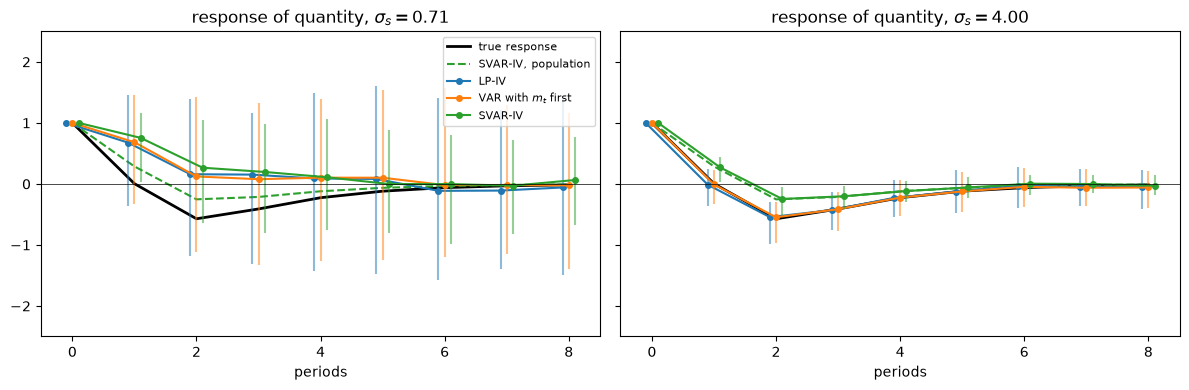
Fig. 30.2 Estimates in samples of 200 periods#
The next cell measures the strength of the instrument by the median, across samples, of the first-stage \(F\) statistic for \(m_t\) in a regression of \(q_t\) on \(m_t\) with the same controls, and computes the response of quantity to a quantity innovation, which is what ordinary least squares would estimate.
def first_stage_F(z, m, p=12):
    "F statistic for the instrument in a regression of q_t on m_t and p lags of (m_t, q_t, p_t)."
    W = np.column_stack([m, z])
    X = np.column_stack([np.ones(len(z) - p), lagged(W, p), m[p:]])
    coef, *_ = np.linalg.lstsq(X, z[p:, 0], rcond=None)
    e = z[p:, 0] - X @ coef
    s2 = e @ e / (len(e) - X.shape[1])
    return coef[-1]**2 / (s2 * np.linalg.inv(X.T @ X)[-1, -1])

rng_F = np.random.default_rng(1)
for σ in [σ_s, 4.0]:
    D_σ = ma_qp(structural_ma(g_s, g_d, φ_A, σ_s=σ))
    F_med = np.median([first_stage_F(*simulate_sample(D_σ, n_obs, rng_F)) for _ in range(n_rep)])
    V_σ, C_σ = wold(D_σ)
    ols = np.array([C_σ[h] @ V_σ[:, 0] / V_σ[0, 0] for h in range(4)])[:, 0]
    print(f"σ_s = {σ:.2f}: median first-stage F {F_med:5.1f};  "
          f"response of q to a quantity innovation, h = 0-3: {np.round(ols, 2)}")
σ_s = 0.71: median first-stage F   1.0;  response of q to a quantity innovation, h = 0-3: [1.   1.37 1.01 0.57]
σ_s = 4.00: median first-stage F  20.4;  response of q to a quantity innovation, h = 0-3: [1.   1.04 0.63 0.34]
With the baseline shock sizes, the instrument is weak: a supply shock moves prices and quantities so little that the median first-stage \(F\) statistic is about 1, far below the rule-of-thumb threshold of 10.
In 200 periods, the local projection and the internal-instrument VAR are then uninformative, and their medians are pulled toward the least-squares response to a quantity innovation, which demand shocks dominate, as estimates with weak instruments typically are; SVAR-IV’s median is pulled the same way, away from even its population value.
With \(\sigma_s = 4\), the instrument is strong, with a median first-stage \(F\) of about 20: the local projection and the internal-instrument VAR are centered on the truth but noisy, while SVAR-IV is more precise and centered on its population value, the dashed line, which is the wrong response.
With few lags, the VAR-based estimators also suffer from truncation: with four lags instead of twelve (not shown), SVAR-IV’s median strays from even its population value, and the internal-instrument VAR’s median drifts from the truth beyond horizon four.
With a strong instrument, the choice between them is a choice between bias and variance: more data shrink the variance of the local projection, but not the bias of SVAR-IV.
30.5. Invertibility depends on the policy rule#
Whether the supply shock is fundamental for \((q_t, p_t)\) is a property of the equilibrium moving-average representation, and that representation depends on the policy rule.
A change in the policy rule can change whether a VAR recovers the supply shock.
φ_grid = np.linspace(-0.5, 10, 22)
fig, ax = plt.subplots()
for g, color in [(3.0, 'C0'), (10.0, 'C1'), (30.0, 'C3')]:
    norms = []
    for φ in φ_grid:
        D = ma_qp(structural_ma(g, g_d, φ))
        V, _ = wold(D)
        norms.append(impulse_norms(D, V)[0])
    ax.plot(φ_grid, norms, 'o-', lw=2, color=color, ms=4, label=f"$g_s = {g:g}$")
ax.axhline(1, color='k', lw=0.5)
ax.axvline(φ_A, color='k', ls=':', lw=1)
ax.set_xlabel("policy rule coefficient $\\phi$")
ax.set_ylabel("$\\|L^{-1} d_s\\|$")
ax.legend()
plt.tight_layout()
plt.show()
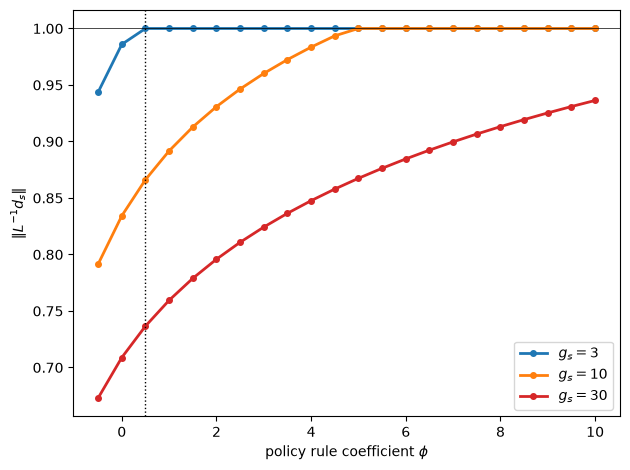
Fig. 30.3 Fundamentalness and the policy rule#
The more aggressively the government stabilizes the price, the closer the supply shock comes to being fundamental.
For \(g_s = 3\) the baseline rule already makes it fundamental, and for \(g_s = 10\) a rule with \(\phi \gtrsim 5\) does; for \(g_s = 30\), a still more aggressive rule would be needed.
A rule that destabilizes the price (\(\phi < 0\)) pushes the economy further from invertibility.
The equivalence of Price stabilization as more flexible supply in Policy Counterfactuals from Impulse Responses explains the pattern.
Under the rule \(\phi\), prices and quantities behave as in a market without a tax whose supplier has cost parameters \(h_s / (1 + \phi)\) and \(g_s / (1 + \phi)\), and whose cost shocks are scaled down by the same factor.
Scaling a shock does not move the zeros of the moving average, so it does not change whether the shock is fundamental.
The rule matters only through the effective cost parameters.
In Exercise 27.2 of Dynamic Supply and Demand Curves we saw that the supply shock becomes fundamental when suppliers can adjust quickly: price stabilization makes them behave as if they could.
The analogy is approximate, because that exercise lowered \(g_s\) with \(h_s\) held fixed, while the rule lowers both.
for φ in [0.5, 2.0]:
    D_rule = ma_qp(structural_ma(g_s, g_d, φ))
    nrm_rule = impulse_norms(D_rule, wold(D_rule)[0])[0]
    D_flex = ma_qp(structural_ma(g_s / (1 + φ), g_d, 0.0, h_s=h_s / (1 + φ), σ_s=σ_s / (1 + φ)))
    nrm_flex = impulse_norms(D_flex, wold(D_flex)[0])[0]
    print(f"φ = {φ}: ||L^-1 d_s|| under the rule {nrm_rule:.4f}, "
          f"in the flexible-supply market {nrm_flex:.4f};  max |D_rule - D_flex| = "
          f"{np.abs(D_rule - D_flex).max():.1e}")
φ = 0.5: ||L^-1 d_s|| under the rule 0.8662, in the flexible-supply market 0.8662;  max |D_rule - D_flex| = 2.0e-15
φ = 2.0: ||L^-1 d_s|| under the rule 0.9308, in the flexible-supply market 0.9308;  max |D_rule - D_flex| = 1.8e-15
The supply shock fails to be fundamental because the moving average \(D(z) = \sum_j D_j z^j\) has a zero inside the unit circle, as in (27.24) of Dynamic Supply and Demand Curves.
We compute the zeros of \(\det D(z)\) that lie inside the unit circle under several rules.
def zeros_inside(D):
    "Zeros of det D(z) = D_11(z) D_22(z) - D_12(z) D_21(z) inside the unit circle."
    poly = np.polynomial.polynomial
    det = poly.polysub(poly.polymul(D[:, 0, 0], D[:, 1, 1]), poly.polymul(D[:, 0, 1], D[:, 1, 0]))
    roots = poly.polyroots(det)
    return roots[np.abs(roots) < 1]

for φ in [0.5, 2.0, 4.0, 6.0]:
    D_φ = ma_qp(structural_ma(g_s, g_d, φ))
    norm = impulse_norms(D_φ, wold(D_φ)[0])[0]
    print(f"φ = {φ}: zeros inside the unit circle {np.round(zeros_inside(D_φ).real, 4)}, "
          f"||L^-1 d_s|| = {norm:.4f}")
φ = 0.5: zeros inside the unit circle [0.8662], ||L^-1 d_s|| = 0.8662
φ = 2.0: zeros inside the unit circle [0.9308], ||L^-1 d_s|| = 0.9308
φ = 4.0: zeros inside the unit circle [0.9835], ||L^-1 d_s|| = 0.9835
φ = 6.0: zeros inside the unit circle [], ||L^-1 d_s|| = 1.0000
Under each rule with a non-fundamental supply shock there is one such zero, and it equals \(\|L^{-1} d_s\|\).
That is no coincidence.
When the moving average has a single zero \(\lambda\) inside the unit circle and the other shock is fundamental, the Wold innovations are the structural shocks with a Blaschke factor applied to the non-fundamental one, and then \(\|L^{-1} d_s\| = |\lambda|\) exactly; here the two agree to within about \(10^{-6}\), because the demand shock is fundamental to that precision.
The \(R^2\) of the projection of the supply shock on current and past data is therefore \(\lambda^2\).
As \(\phi\) rises, the zero moves toward the unit circle, and somewhere between \(\phi = 4\) and \(\phi = 6\) it crosses it.
This is a version of the Lucas critique that applies to identification: a VAR identification scheme that is valid under one policy regime can fail under another, because the zeros of the equilibrium moving-average representation move with the policy rule.
30.6. Counterfactual second moments through VAR innovations#
McKay and Wolf also predict the unconditional second moments of the data under a new rule.
If the econometrician could identify every structural shock, she could apply Proposition 1 to each one and add up the resulting variances and autocovariances.
When the structural shocks cannot all be identified, McKay and Wolf propose applying Proposition 1 to the impulse responses of the Wold innovations instead, and they show that this is valid if the structural moving-average representation is invertible.
We compare the Wold-innovation route with the true counterfactual autocovariances.
def autocov(X, n_lags=12):
    "Autocovariances Γ_j (3 x 3), j = 0..n_lags, from stacked impulse responses X (3T x k)."
    P = np.stack([X[b * T:(b + 1) * T] for b in range(3)])     # 3 x T x k
    return np.array([np.einsum('itk,jtk->ij', P[:, j:], P[:, :T - j])
                     for j in range(n_lags + 1)])

def wold_route(g_s_, φ_base, φ_cf, σ_s_=σ_s):
    "Counterfactual autocovariances: truth versus the Wold-innovation route."
    M_inv_base = system_inverse(g_s_, g_d, φ_base)
    X_base = np.stack([M_inv_base @ forcing(k, σ_s=σ_s_) for k in range(2)], axis=1)
    X_true = structural_ma(g_s_, g_d, φ_cf, σ_s=σ_s_)
    D = ma_qp(X_base)
    V, C_wold = wold(D)
    W = C_wold[:H_ma] @ np.linalg.cholesky(V)       # responses to orthonormal Wold innovations
    X_w = []
    for k in range(2):
        q, p = np.zeros(T), np.zeros(T)
        q[:H_ma], p[:H_ma] = W[:, 0, k], W[:, 1, k]
        x_k, _ = mw_counterfactual(M_inv_base, np.concatenate([q, p, -φ_base * p]), φ_cf)
        X_w.append(x_k)
    X_w = np.stack(X_w, axis=1)
    Γ_true, Γ_w = autocov(X_true), autocov(X_w)
    return Γ_true, Γ_w, impulse_norms(D, V)[0]

print(" g_s   ||L^-1 d_s||   var(q): true   Wold route   max relative error in Γ_0..Γ_12")
for g in [0.5, 10.0]:
    Γ_true, Γ_w, nrm = wold_route(g, φ_A, φ_new)
    rel = np.abs(Γ_w - Γ_true).max() / np.abs(Γ_true).max()
    print(f"{g:4.1f}  {nrm:12.4f}  {Γ_true[0, 0, 0]:13.5f}  {Γ_w[0, 0, 0]:11.5f}  {rel:22.1e}")
 g_s   ||L^-1 d_s||   var(q): true   Wold route   max relative error in Γ_0..Γ_12
 0.5        1.0000        3.01567      3.01567                 1.2e-15
10.0        0.8662        0.89802      0.89804                 2.5e-05
The last column is the largest error in any autocovariance of \((q, p, \tau)\) at lags 0 to 12, relative to the largest autocovariance.
When the supply shock is fundamental (\(g_s = 0.5\)), the Wold-innovation route reproduces the true counterfactual autocovariances to machine precision.
When it is not (\(g_s = 10\)), the route makes an error, but the error is tiny.
30.6.1. Why the route errs#
Invertibility makes the route exact for the following reason.
Under invertibility, each Wold innovation is a linear combination of the current structural shocks, and its impulse response is a linear combination of date-0 structural impulse responses, to which (30.1) applies.
Under non-invertibility, a Wold innovation also contains past structural shocks, and its impulse response includes the continuations of paths that started before date 0.
Write \(u_t = \sum_{j \ge 0} K_j \epsilon_{t-j}\) for the Wold innovations in terms of the structural shocks, with \(K_0 = D_0\).
We compute the weights \(K_j\), \(j \ge 1\), on past shocks.
K_w = np.zeros_like(D_A)                  # u_t = Σ_j K_j ε_(t-j)
for k in range(H_ma):
    K_w[k] = D_A[k] - sum(C_wold_A[j] @ K_w[k - j] for j in range(1, k + 1))
print(f"largest weight on past supply shocks {np.abs(K_w[1:, :, 0]).max():.4f}, "
      f"on past demand shocks {np.abs(K_w[1:, :, 1]).max():.1e}")
largest weight on past supply shocks 0.0114, on past demand shocks 2.5e-05
Only past supply shocks enter, because the demand shock is fundamental.
The past supply shocks in the Wold innovations are not negligible relative to the current one.
With a single zero \(\lambda\) inside the unit circle, the supply part of the orthonormalized innovation is the Blaschke-filtered shock \(\lambda \epsilon_{st} - (1 - \lambda^2) \sum_{j \ge 1} \lambda^{j-1} \epsilon_{s,t-j}\), so the weights on past shocks decay at the rate \(\lambda \approx 0.866\), and together they carry \((1 - \lambda^2) / \lambda^2 \approx 1/3\) as much variance as the weight on the current shock.
Proposition 1 treats the continuation of a supply-shock path that started before date 0 as a fresh date-0 path from the steady state, ignoring that agents had already been responding to it, and so maps it incorrectly.
X_new_struct = structural_ma(g_s, g_d, φ_new)

def continuation(x, k):
    "The part of each path (q, p, τ) from date k on, restarted at date 0."
    out = np.zeros_like(x)
    for b in range(3):
        out[b * T:(b + 1) * T - k] = x[b * T + k:(b + 1) * T]
    return out

peak = [np.abs(split(X_new_struct[:, 0])[i]).max() for i in range(2)]
print("continuation from date k: max |mapped - true| relative to the peak of the true response")
for k in range(1, 9):
    mapped, _ = mw_counterfactual(M_inv_A, continuation(X_A[:, 0], k), φ_new)
    target = continuation(X_new_struct[:, 0], k)
    rel = [np.abs(split(mapped)[i] - split(target)[i])[:T - 10].max() / peak[i] for i in range(2)]
    print(f"  k = {k}:  q {rel[0]:.3f},  p {rel[1]:.3f}")
continuation from date k: max |mapped - true| relative to the peak of the true response
  k = 1:  q 0.037,  p 0.053
  k = 2:  q 0.001,  p 0.007
  k = 3:  q 0.040,  p 0.052
  k = 4:  q 0.048,  p 0.075
  k = 5:  q 0.041,  p 0.072
  k = 6:  q 0.030,  p 0.057
  k = 7:  q 0.019,  p 0.040
  k = 8:  q 0.011,  p 0.025
Proposition 1 misses these continuations by up to about 7.5 percent of the peak of the true response; the misses are largest near \(k = 4\) and fade gradually, to 1 to 2.5 percent by \(k = 8\).
The continuation from date 2 is the exception: one period after a supply shock, quantity is almost exactly at its steady state under both rules, so that continuation starts from nearly the state that Proposition 1 assumes.
The error comes from the state that a continuation inherits.
That is one source of error; there is a second.
The response of the baseline outcomes \(z_{t+h}\) to the Wold innovation \(u_t\) is determined by their covariance with it,
and under the baseline rule this sum is zero for \(h < 0\), because \(u_t\) is uncorrelated with past data.
Under the counterfactual rule, the same sum with the counterfactual structural responses \(\tilde D_h\) in place of \(D_h\) is not zero for \(h < 0\): the weights \(K_j\) make the past supply shocks in \(u_t\) cancel against past baseline outcomes, but they do not cancel against past counterfactual outcomes.
So the counterfactual outcomes are not a one-sided moving average of the baseline Wold innovations, and the Wold-innovation route, which builds such a moving average, leaves out the pieces dated before the innovation.
Write \(\tilde R_h = \sum_{j \ge 0} \tilde D_{h+j} K_j^\top\) for these covariances under the counterfactual rule.
Because the two-sided history of the Wold innovations spans the two-sided history of the structural shocks, the counterfactual outcomes are \(\tilde z_t = \sum_{h = -\infty}^{\infty} \tilde R_h V^{-1} u_{t-h}\), and their autocovariances are
The next cell computes this sum first over \(h \ge 0\) only, which uses the true continuations in place of Proposition 1’s, and then over all \(h\).
D_new = np.stack([X_new_struct[b * T:(b + 1) * T] for b in range(3)], axis=1)   # T x 3 x 2

D_base = np.stack([X_A[b * T:(b + 1) * T] for b in range(3)], axis=1)      # T x 3 x 2

def cov_with_u(D_paths, h):
    "Σ_j D_(h+j) K_j^T: covariance of the outcomes (q, p, τ)_(t+h) with the baseline Wold innovation u_t."
    return sum((D_paths[h + j] @ K_w[j].T for j in range(H_ma) if 0 <= h + j < T), np.zeros((3, 2)))

R_u = {h: cov_with_u(D_new, h) for h in range(-H_ma, T)}
V_A_inv = np.linalg.inv(V_A)

def autocov_from(hs, n_lags=12):
    return np.array([sum(R_u[h + j] @ V_A_inv @ R_u[h].T for h in hs if h + j in R_u)
                     for j in range(n_lags + 1)])

Γ_new = autocov(X_new_struct)
_, Γ_route, _ = wold_route(g_s, φ_A, φ_new)
print("                                  max relative error in Γ_0..Γ_12   error in var(q) / var(q)")
for label, Γ_h in [("Wold-innovation route", Γ_route),
                   ("true continuations, h >= 0 only", autocov_from(range(0, T))),
                   ("adding the pieces with h < 0", autocov_from(range(-H_ma, T)))]:
    err = np.abs(Γ_h - Γ_new).max() / np.abs(Γ_new).max()
    err_q = (Γ_h[0, 0, 0] - Γ_new[0, 0, 0]) / Γ_new[0, 0, 0]
    print(f"{label:32s}  {err:21.1e}   {err_q:24.1e}")
print(f"largest covariance with h < 0: counterfactual {max(np.abs(R_u[h]).max() for h in range(-H_ma, 0)):.1e}, "
      f"baseline {max(np.abs(cov_with_u(D_base, h)).max() for h in range(-H_ma, 0)):.1e};  "
      f"largest with h >= 0: {max(np.abs(R_u[h]).max() for h in range(T)):.1f}")
                                  max relative error in Γ_0..Γ_12   error in var(q) / var(q)
Wold-innovation route                           2.5e-05                    2.9e-05
true continuations, h >= 0 only                 2.4e-05                   -4.9e-06
adding the pieces with h < 0                    1.7e-14                    2.4e-14
largest covariance with h < 0: counterfactual 2.0e-04, baseline 7.8e-09;  largest with h >= 0: 4.4
The two sources of error matter at different lags.
With the true continuations in place of Proposition 1’s, the error in the variance of quantity falls by more than four fifths, but the largest error, which is in autocovariances at lags one and two, barely changes; adding the pieces dated before the innovation removes the error entirely.
Caravello et al. [2026] (Appendix A.6) discuss the problem in lag-operator notation.
In their notation, the covariances \(\tilde R_h\) are, up to the normalization of the innovations, the coefficients of \(\tilde \Theta(L) P^*(L^{-1})\), and the pieces with \(h < 0\) are its negative powers of \(L\).
They locate the failure in \(P^*(L^{-1}) P(L) \neq I\), which must occur when there are more shocks than observables, as in their application to the model of Smets and Wouters [2007].
In our market, with two shocks and two observables, \(P^*(L^{-1}) P(L) = I\) (which is what makes the two-sided sum above exact), so the failure lies elsewhere: the route’s responses are not \(\tilde \Theta(L) P^*(L^{-1})\), because they mis-map the continuations and leave out the pieces with \(h < 0\).
30.6.2. Why the error is small#
The overall error is tiny because supply shocks account for very little of the variance of prices and quantities.
var_by_shock = (D_A**2).sum(axis=0)               # rows: (q, p); columns: (supply, demand)
share = var_by_shock[:, 0] / var_by_shock.sum(axis=1)
print(f"share of the variance due to supply shocks: q {share[0]:.4f}, p {share[1]:.4f}")
share of the variance due to supply shocks: q 0.0037, p 0.0004
Supply shocks account for less than 0.4 percent of the variance of quantity and less than 0.05 percent of the variance of price, a feature of our calibration that Exercise 30.1 relaxes.
Caravello et al. [2026] show what the Wold-innovation route requires.
Following Barnichon and Mesters [2023], they prove that the Wold representation suffices for counterfactual second moments if and only if the forecasts it implies equal full-information forecasts, those based on the whole history of shocks.
Invertibility is sufficient, but not necessary.
The approximate version of their result is that the route is accurate when forecasts based on the econometrician’s information — here, the history of prices and quantities — are close to full-information forecasts.
We compare the variances of \(h\)-step-ahead forecast errors under the two information sets.
print(" h    forecast-error variance, (q, p) history / full information")
print("          quantity      price")
for h in [1, 2, 4, 8]:
    full = sum(D_A[j] @ D_A[j].T for j in range(h))
    obs = sum(C_wold_A[j] @ V_A @ C_wold_A[j].T for j in range(h))
    print(f"{h:2d}   {obs[0, 0] / full[0, 0]:12.4f} {obs[1, 1] / full[1, 1]:10.4f}")
 h    forecast-error variance, (q, p) history / full information
          quantity      price
 1         1.0033     1.0002
 2         1.0015     1.0002
 4         1.0001     1.0000
 8         1.0000     1.0000
Forecasts based on prices and quantities are at most a third of a percent worse than forecasts based on the shocks themselves.
The two ways of describing the error, the weights \(K_j\) on past shocks and the ratios of forecast-error variances, coincide at \(h = 1\).
The one-step forecast error under the econometrician’s information is \(u_t\), and under full information it is \(D_0 \epsilon_t\); the excess variance \(V - D_0 D_0^\top = \sum_{j \ge 1} K_j K_j^\top\) is exactly the variance that the weights on past shocks contribute.
So the first row of the table measures those weights: they add 0.33 percent to the full-information forecast-error variance of quantity and 0.02 percent to that of price.
Caravello et al. [2026] find accurate counterfactual second moments in the model of Smets and Wouters [2007] even with three observables and seven shocks, far from invertibility, where forecast-error variances are at most around 12 percent larger than with full information.
30.7. Summary#
Our market sorts procedures by whether they need invertibility.
procedure |
needs invertibility? |
in this market, \(g_s = 10\) |
|---|---|---|
Cholesky or sign-restricted rotations of VAR innovations |
yes |
miss the supply-shock response |
SVAR-IV (“external instrument”): the instrument selects a rotation of VAR innovations |
yes |
right direction on impact but size overstated by about 15 percent; wrong afterward |
local projection on an instrument (LP-IV), or a VAR with the instrument ordered first |
no |
recovers the supply-shock response |
McKay–Wolf counterfactual for a given shock (Proposition 1), with impulse responses from LP-IV |
no |
exact in population |
McKay–Wolf counterfactual second moments via Wold innovations |
sufficient, not necessary: exact if and only if Wold forecasts equal full-information forecasts |
small error, because forecasts from \((q, p)\) are nearly as good as full-information forecasts |
The first three rows concern identification under the baseline rule.
The last two presume McKay and Wolf’s environment: a linear private sector, a credible counterfactual rule, and policy shocks that do not change beliefs about the rule (McKay and Wolf and dynamic programming squared of Policy Counterfactuals from Impulse Responses).
First, invertibility is not a fixed property of an economy: it depends on the policy rule, and a VAR identification scheme that works under one regime can fail under another — in our market because price stabilization acts like a proportional reduction in suppliers’ production and adjustment costs.
Second, in this market, non-invertibility matters a great deal for some objects — the impulse response to the supply shock — and very little for others — counterfactual second moments, partly because supply shocks account for so little of the variance of prices and quantities.
Third, the methods that do not need invertibility pay for it in samples of realistic length: in 200 periods, local projections on the instrument are noisy even when the instrument is strong, though then centered on the truth, and with our calibration the instrument is so weak that they are uninformative and median-biased.
30.8. Exercises#
Exercise 30.1
The error that the Wold-innovation route makes under non-invertibility is small in our market partly because the non-fundamental supply shock contributes little to the variance of prices and quantities.
Recompute the table of counterfactual second moments with \(g_s = 10\) and larger supply-shock standard deviations, \(\sigma_s \in \{2, 4, 8, 16, 32\}\).
How do the error, the share of the variance of quantity due to supply shocks, and the ratio of one-step forecast-error variances change?
Solution
print(" σ_s   ||L^-1 d_s||   ||L^-1 d_d||   supply share of var(q)   max relative error in Γ_0..Γ_12   one-step ratio for q")
for σ in [np.sqrt(0.5), 2.0, 4.0, 8.0, 16.0, 32.0]:
    Γ_true, Γ_w, nrm = wold_route(10.0, φ_A, φ_new, σ_s_=σ)
    rel = np.abs(Γ_w - Γ_true).max() / np.abs(Γ_true).max()
    D_σ = ma_qp(structural_ma(10.0, g_d, φ_A, σ_s=σ))
    V_σ, _ = wold(D_σ)
    share_q = (D_σ[:, 0, 0]**2).sum() / (D_σ[:, 0, :]**2).sum()
    ratio = V_σ[0, 0] / (D_σ[0] @ D_σ[0].T)[0, 0]
    nrm_d = impulse_norms(D_σ, V_σ)[1]
    print(f"{σ:5.2f}  {nrm:12.4f}  {nrm_d:12.4f}  {share_q:23.3f}  {rel:32.1e}  {ratio:20.4f}")
 σ_s   ||L^-1 d_s||   ||L^-1 d_d||   supply share of var(q)   max relative error in Γ_0..Γ_12   one-step ratio for q
 0.71        0.8662        1.0000                    0.004                           2.5e-05                1.0033
 2.00        0.8662        1.0000                    0.029                           2.0e-04                1.0249
 4.00        0.8662        1.0000                    0.107                           7.9e-04                1.0807
 8.00        0.8663        0.9999                    0.323                           3.0e-03                1.1833
16.00        0.8665        0.9997                    0.657                           1.0e-02                1.2686
32.00        0.8676        0.9988                    0.884                           2.7e-02                1.3019
The zero of \(\det D(z)\) does not move, because scaling a column of \(D(z)\) does not change its zeros, and \(\|L^{-1} d_s\|\) barely changes: a larger \(\sigma_s\) scales up the supply shock’s contribution to the data without making supply surprises any easier to detect.
It does rise slightly, because the demand shock is not exactly fundamental: the direction that the data fail to reveal is almost entirely the supply shock but has a small demand component, and as supply shocks come to dominate the data that component grows, so that \(\|L^{-1} d_d\|\) falls further below one and \(\|L^{-1} d_s\|\) rises.
While supply shocks account for a small share of the variance, the error grows roughly in proportion to \(\sigma_s^2\), because the part of the Wold innovations that reflects past supply shocks gets more weight.
It then grows more slowly, and even when supply shocks account for nearly 90 percent of the variance of quantity, the largest error in an autocovariance is below 3 percent of the largest autocovariance, although forecasts based on prices and quantities are then about 30 percent worse than full-information forecasts.
Relative to their own size, entries differ: with \(\sigma_s = 32\), the variance of quantity is off by 1.5 percent, that of price by 1.7 percent, and their covariance, which is smaller, by 5.6 percent.
In this market the Wold-innovation route stays accurate far from invertibility, consistent with the findings of Caravello et al. [2026] for the model of Smets and Wouters [2007].
Exercise 30.2
In Induced Priors for Impulse Responses, sign restrictions that the theory implies with prior probability one identified a set of supply-shock responses that excluded the true response, because the supply shock is not fundamental.
We have seen that a sufficiently aggressive price-stabilizing rule makes the supply shock fundamental.
For the rules \(\phi = 0.5\) and \(\phi = 6\), compute the signs of the responses of \((q, p)\) to the two shocks at horizons \(0, \ldots, 5\) that hold for every draw from the prior \(g_s \sim U[8, 12]\), \(g_d \sim U[0.05, 0.15]\).
For each rule, give the econometrician the population VAR at the true parameters, impose those sign restrictions on rotations of the VAR innovations, and check whether the identified set of supply-shock responses contains the truth.
Solution
We compute the sign table from 150 prior draws and then sweep over rotations of the VAR innovations, normalizing each shock to raise quantity on impact, as in Induced Priors for Impulse Responses.
K_signs = 5
angles = np.linspace(0, 2 * np.pi, 20_000, endpoint=False)

def theory_sign_table(φ, n=150, seed=0):
    "Signs of the responses of (q, p) that hold for every prior draw: +1, -1, or 0."
    rng = np.random.default_rng(seed)
    draws = []
    for _ in range(n):
        g_s_i, g_d_i = rng.uniform(8, 12), rng.uniform(0.05, 0.15)
        M = np.vstack([private_block(g_s_i, g_d_i), rule_block(φ)])
        X = np.linalg.solve(M, np.column_stack([forcing(0), forcing(1)]))
        draws.append(ma_qp(X)[:K_signs + 1])
    draws = np.array(draws)
    return np.where((draws > 0).all(0), 1, np.where((draws < 0).all(0), -1, 0))

tables = {φ: theory_sign_table(φ) for φ in [0.5, 6.0]}
symbol = {1: '+', -1: '-', 0: '?'}
for φ, table in tables.items():
    print(f"sign table under φ = {φ} (rows: horizons 0-{K_signs}; columns: q|s, p|s, q|d, p|d)")
    for h in range(K_signs + 1):
        print("   ", h, " ".join(symbol[table[h, i, k]] for k in range(2) for i in range(2)))
print("entries that differ:", int((tables[0.5] != tables[6.0]).sum()))

fig, axes = plt.subplots(2, 2, figsize=(12, 7))
for col, φ in enumerate([0.5, 6.0]):
    table = tables[φ]
    D = ma_qp(structural_ma(g_s, g_d, φ))
    V, C_w = wold(D)
    L = np.linalg.cholesky(V)
    r1 = L @ np.vstack([np.cos(angles), np.sin(angles)])
    r2 = L @ np.vstack([-np.sin(angles), np.cos(angles)])
    r1, r2 = r1 * np.sign(r1[0]), r2 * np.sign(r2[0])   # each shock raises q on impact
    supply = np.einsum('tij,jm->tim', C_w[:H_plot], r1)
    demand = np.einsum('tij,jm->tim', C_w[:H_plot], r2)
    ok = (np.all(supply[:K_signs + 1] * table[:, :, [0]] >= 0, axis=(0, 1))
          & np.all(demand[:K_signs + 1] * table[:, :, [1]] >= 0, axis=(0, 1)))
    lo, hi = supply[:, :, ok].min(axis=2), supply[:, :, ok].max(axis=2)
    inside = (lo - 1e-10 <= D[:H_plot, :, 0]) & (D[:H_plot, :, 0] <= hi + 1e-10)
    print(f"φ = {φ}: ||L^-1 d_s|| = {impulse_norms(D, V)[0]:.3f}, "
          f"share of rotations kept = {ok.mean():.4f}, "
          f"truth inside the set: q {inside[:, 0].all()}, p {inside[:, 1].all()}")
    for i in range(2):
        ax = axes[i, col]
        ax.fill_between(range(H_plot), lo[:, i], hi[:, i], color='C3', alpha=0.3,
                        label=f"sign-identified set, K = {K_signs}")
        ax.plot(D[:H_plot, i, 0], 'k--', lw=2, label="true supply-shock response")
        ax.axhline(0, color='k', lw=0.5)
        ax.set_title(f"{names[i]}, supply shock, $\\phi = {φ}$")
        ax.set_xlim(0, 12)
axes[0, 0].legend(fontsize=8)
plt.tight_layout()
plt.show()
sign table under φ = 0.5 (rows: horizons 0-5; columns: q|s, p|s, q|d, p|d)
    0 + - + +
    1 ? ? + +
    2 - + + +
    3 - + + -
    4 - + + -
    5 - + + -
sign table under φ = 6.0 (rows: horizons 0-5; columns: q|s, p|s, q|d, p|d)
    0 + - + +
    1 - ? + +
    2 - + + ?
    3 - + + -
    4 - + ? -
    5 ? + ? -
entries that differ: 5
φ = 0.5: ||L^-1 d_s|| = 0.866, share of rotations kept = 0.0160, truth inside the set: q False, p False
φ = 6.0: ||L^-1 d_s|| = 1.000, share of rotations kept = 0.0106, truth inside the set: q True, p True
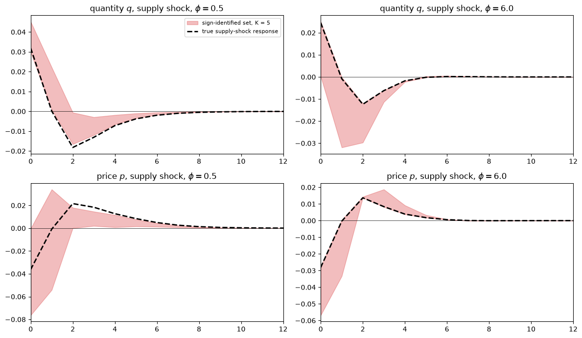
Under the baseline rule the supply shock is not fundamental, and the theory-implied sign restrictions identify a set that misses the true response, just as in Induced Priors for Impulse Responses.
Under the aggressive rule the supply shock is fundamental, the true response is one of the admissible rotations, and the identified set contains it.
The sign table itself changes with the rule: a ? marks a sign that the theory leaves open, and the
printed tables differ in several entries, including the response of quantity to a supply shock one period
after impact.
The theory’s sign implications are properties of an equilibrium and are subject to the Lucas critique.
Exercise 30.3
Plagborg-Møller and Wolf [2022] show that an instrument can test invertibility.
Under invertibility, the Wold innovations at dates after \(t\) are combinations of structural shocks after \(t\), so the instrument \(m_t\) is uncorrelated with \(u_{t+j}\) for every \(j \ge 1\); under non-invertibility, \(u_{t+j}\) contains the date-\(t\) supply shock and the correlation need not be zero.
Using the weights \(K_j\) of the Wold innovations on past shocks, compute the correlations between \(m_t\) and \(u_{t+j}\), \(j = 1, 2, 3\), under the rules \(\phi = 0.5\) and \(\phi = 6\).
Roughly how long a sample would be needed for a test at the 5 percent level to detect the largest of these correlations under \(\phi = 0.5\)?
Solution
The correlation between \(m_t = \epsilon_{st} + v_t\) and the \(i\)th element of \(u_{t+j}\) is the supply column of \(K_j\), divided by the standard deviation of \(m_t\), which is \(\sqrt{2}\), and by that of the innovation.
def wold_weights(D):
    "Innovation covariance V and weights K_j in u_t = Σ_j K_j ε_(t-j)."
    V, C_w = wold(D)
    K = np.zeros_like(D)
    for k in range(H_ma):
        K[k] = D[k] - sum(C_w[j] @ K[k - j] for j in range(1, k + 1))
    return V, K

for φ in [0.5, 6.0]:
    V_φ, K_φ = wold_weights(ma_qp(structural_ma(g_s, g_d, φ)))
    corr = np.array([K_φ[j][:, 0] / np.sqrt(2 * np.diag(V_φ)) for j in range(1, 4)])
    corr = np.round(corr, 4) + 0.0           # + 0.0 turns -0.0 into 0.0
    print(f"φ = {φ}: corr(m_t, u_(t+j)) for j = 1, 2, 3, quantity {corr[:, 0]}, price {corr[:, 1]}")
φ = 0.5: corr(m_t, u_(t+j)) for j = 1, 2, 3, quantity [-0.0204 -0.0177 -0.0153], price [0.0053 0.0046 0.004 ]
φ = 6.0: corr(m_t, u_(t+j)) for j = 1, 2, 3, quantity [0. 0. 0.], price [0. 0. 0.]
Under the aggressive rule, which makes the supply shock fundamental, the correlations are zero.
Under the baseline rule they are not, but they are small: the largest is about 0.02 in absolute value.
A sample correlation has a standard error of about \(1/\sqrt{n}\), so in a sample of \((1.96/0.02)^2 \approx 10{,}000\) periods a correlation of 0.02 is, on average, just significant at the 5 percent level, and a test detects it only half the time; detecting it with probability 0.8 takes about \(((1.96 + 0.84)/0.02)^2 \approx 20{,}000\) periods.
A joint test of the correlations at several leads needs fewer, because the correlations decay slowly.
The test is informative in principle and weak in this market for the same reason that the Wold-innovation route is accurate: the non-fundamental supply shock contributes little to the data.