72. Gradual Liberalization in a Global Production Network#
72.1. Overview#
Institution Building Without Commitment computed organizational equilibrium tariffs in the two-country, two-sector model of Bassetto et al. [2024].
Bassetto et al. [2026] take the same question to a quantitative model of the G7 economies with 30 sectors, trade in final and intermediate goods, workers attached to sectors, and internationally mobile capital.
Two ideas make their model tractable.
Static separability: every static quantity is proportional to the world capital stock, so the dynamic policy problem depends on the static economy only through two functions of the tariff, worker welfare \(\chi(\tau)\) and the gross return to capital \(G(\tau)\), just as in Institution Building Without Commitment.
Exact hat algebra: \(\chi(\tau)\) and \(G(\tau)\) can be computed from observed expenditure and production shares, without estimating technologies, tastes, or the sizes of labor forces [Dekle et al., 2008].
Their model belongs to a family of global production network models that Huo et al. [2025] use to study how business cycles spread across countries and that Bonadio et al. [2026] use to quantify the recent reorganization of world trade into blocs.
This lecture builds a small version of the model, with three countries and five sectors.
We do not use the data of Bassetto et al. [2026].
Instead we use illustrative shares, chosen so that the model’s Markov and best constant tariffs, 14.5 and 1.2 percent, are close to theirs, about 12 and 1.3 percent.
Matching their tariffs requires wages to be very unequal across home’s sectors, and we explain why.
The lecture
sets out the model, shows why it is separable, and solves it in changes from a baseline,
decomposes how a tariff affects the welfare of home’s workers,
derives a simple condition that tells when a tariff is worth its cost to capital accumulation,
computes Markov, Ramsey, and organizational equilibrium tariffs and their responses to a protectionist shock, and
relates the model to the recent formation of trade blocs.
We use the following imports.
import numpy as np
import matplotlib.pyplot as plt
from collections import namedtuple
from scipy.interpolate import CubicSpline
from scipy.optimize import brentq, minimize, minimize_scalar
72.2. The economy#
There are \(N\) countries, indexed by \(m\) and \(n\), and \(J\) sectors, indexed by \(i\) and \(j\).
Each country-sector pair produces a distinct good, so buyers treat goods from different countries as imperfect substitutes [Armington, 1969].
Time is discrete, and we drop time subscripts when nothing is lost.
72.2.1. Tariffs#
A lead country, which we call home and number \(1\), chooses a tariff \(\tau\) on all imports, and every other country responds with the same tariff on its own imports.
A buyer in country \(n\) therefore pays \(D_{mn} p_{mj}\) for a sector-\(j\) good that sells for \(p_{mj}\) in country \(m\), where
is the gross tariff wedge.
72.2.2. Final goods#
Country \(n\)’s final good, which is used for both consumption and investment, is a Cobb–Douglas aggregate of sector bundles with expenditure shares \(\Phi_j\).
Each sector bundle is a CES aggregate of the goods of all origins with elasticity of substitution \(\varepsilon\).
The price of country \(n\)’s final good is
where the weights \(\Omega^c_{mnj}\) capture tastes and trade costs other than tariffs.
Origin \(m\) receives the share
of country \(n\)’s final spending on sector \(j\).
72.2.3. Production#
Sector \(j\) in country \(n\) produces with capital \(k_{nj}\), labor \(\ell_{nj}\), and a bundle \(x_{nj}\) of intermediate inputs, where labor equals the fixed number \(L_{nj}\) of workers attached to the sector:
where \(K_n = \sum_j k_{nj}\) is the capital stock used in country \(n\), which firms take as given.
This externality makes output proportional to capital, as in an \(AK\) growth model.
The input bundle \(x_{nj}\) is a Cobb–Douglas aggregate of sector bundles with shares \(\Xi_{ji}\), and each sector bundle is a CES aggregate across origins with the same elasticity \(\varepsilon\).
For simplicity, all buyers of inputs from sector \(i\) in country \(n\) split their purchases across origins in the same shares \(\pi^x_{mni}\).
Let \(e_{nj} = p_{nj} y_{nj}\) be the revenue of sector \(j\) in country \(n\).
Cost minimization gives
where \(R\) is the rental rate of capital, \(W_{nj}\) is the wage in sector \(j\) of country \(n\), and \(P^x_{nj}\) is the price of the input bundle.
72.2.4. Workers#
Workers are attached to their sector and do not save.
Each worker receives an equal share of the country’s tariff revenue \(T_n = T^c_n + T^x_n\), collected on imports of final goods and of intermediate inputs, so a worker in sector \(j\) of country \(n\) consumes
where \(L_n = \sum_j L_{nj}\).
72.2.5. The world capitalist#
A world capitalist owns the world capital stock \(K\) and rents it to firms in all countries at the common rate \(R\).
The capitalist buys a Cobb–Douglas composite of the countries’ final goods with expenditure shares \(\mu_n\) and price \(P^K = \prod_n P_n^{\mu_n}\), and divides it between consumption \(C^K\) and new capital:
where \(\delta_k\) is the depreciation rate.
The capitalist maximizes \(\sum_t \beta^t (C^K_t)^{1 - \sigma} / (1 - \sigma)\), which gives the same Euler equation for the saving rate \(s_t = K_{t+1} / (G_t K_t)\) as in Institution Building Without Commitment.
The capitalist’s spending on final goods, \(R K\), is divided across countries in the proportions \(\mu_n\).
72.2.6. The policymaker#
Home’s policymaker maximizes the welfare of home’s workers,
where \(\lambda_j = L_{1j} / L_1\) is the share of home’s workers employed in sector \(j\).
72.3. Static equilibrium and separability#
Given the tariff and the world capital stock, a static equilibrium is a set of prices and allocations at which firms and buyers optimize and all markets clear.
Country \(n\)’s spending on final goods consists of its workers’ income and the capitalist’s spending there,
Tariff revenues are
The revenue of each country-sector equals what buyers spend on its good, net of tariffs:
Given the shares, (72.1) is a homogeneous linear system in revenues, so we normalize world revenue to \(\sum_{n, j} e_{nj} = 1\).
Bassetto et al. [2026] show that the static equilibrium is separable in world capital.
Suppose we multiply the world capital stock by \(a > 0\), multiply every quantity of capital, inputs, and output by \(a\), divide every price by \(a\), and leave wages unchanged.
Because the externality makes each production function homogeneous of degree one in capital, inputs, and the country’s capital stock, the scaled quantities are feasible.
Because all goods prices and the rental rate move together, no expenditure share changes, and revenues, wages, and tariff revenues are unchanged.
So revenues, shares, and tariff revenues depend on the tariff but not on \(K\), and prices are proportional to \(1/K\).
It follows that each worker’s consumption is proportional to world capital, \(C_{nj} = K \psi_{nj}(\tau)\), and that the real rental rate \(r = R / P^K\) depends only on the tariff.
The policymaker’s payoff therefore has the form that it has in Institution Building Without Commitment,
with \(\chi(\tau) = \sum_j \lambda_j \log \psi_{1j}(\tau)\) and \(G(\tau) = 1 + r(\tau) - \delta_k\).
Once we know \(\chi\) and \(G\), everything in that lecture’s analysis of tariffs carries over.
72.4. Solving in changes#
Bassetto et al. [2026] compute \(\chi\) and \(G\) by solving the static equilibrium in changes from a baseline equilibrium with tariff \(\tau_0\).
Write \(\hat z = z' / z\) for the ratio of a variable’s value at a new tariff to its value at the baseline, and let \(d_{mn} = D'_{mn} / D_{mn}\).
Origin shares and price indices for final goods change according to
and those for intermediate inputs change in the same way.
The weights \(\Omega^c_{mnj}\) have dropped out, because baseline shares summarize them.
Solving the production function for the price at which revenue \(e_{nj}\) is consistent with cost minimization, and dividing by its baseline value, gives
where \(\vartheta_n = \sum_j \alpha_{k, j} e_{nj} / \kappa\) is country \(n\)’s share of world capital; the technologies \(A_{nj}\) and the numbers of workers \(L_{nj}\) have dropped out too.
Given baseline shares and revenues, the new shares, (72.2), and (72.1) determine the new equilibrium, which we compute by iterating on prices and revenues.
Worker welfare needs only home’s employment shares, since \(\psi_{1j} \propto (\alpha_{\ell, j} e_{1j} / \lambda_j + T_1) / P_1\), with a factor of proportionality that is the same for all sectors.
The gross return needs one more number, the baseline real rental rate \(r_0\), because the changes give only \(r(\tau) / r_0\).
Like Bassetto et al. [2026], we choose \(r_0\) so that capital grows at 2 percent a year in the long run of the organizational equilibrium.
72.5. How tariffs affect home’s workers#
We solve the model on a grid of common tariffs and record what \(\chi\) and \(G\) need: home’s wages, its tariff revenues, its price level, and the real return to capital relative to the baseline, \(\rho(\tau) = r(\tau) / r_0\).
τ_grid = np.linspace(0, 0.6, 121)
κ_0 = (model.α_k * model.e).sum()
wages, T_c, T_x, P_home, ρ = [], [], [], [], []
start = None
for τ in τ_grid:
    eq = solve_changes(tariff_wedges(τ), model, start)
    start = (eq['p'], eq['e'])                     # warm start for the next tariff
    wages.append(model.α_l * eq['e'][0] / model.λ)  # L_1 times each sector's wage
    T_c.append(eq['T_c'][0])
    T_x.append(eq['T_x'][0])
    P_home.append(eq['P'][0])
    ρ.append(eq['κ'] / κ_0 / np.exp(model.μ @ np.log(eq['P'])))
wages, T_c, T_x, P_home, ρ = map(np.array, (wages, T_c, T_x, P_home, ρ))

λ = model.λ
ψ = (wages + (T_c + T_x)[:, None]) / P_home[:, None]   # consumption, up to a constant
χ_grid = np.log(ψ) @ λ
χ_s, ρ_s = CubicSpline(τ_grid, χ_grid), CubicSpline(τ_grid, ρ)
Bassetto et al. [2026] decompose the change in \(\chi\) in two ways.
The first separates the change in workers’ real wages from the rebates of the two kinds of tariff revenue.
Let \(f(T) = \sum_j \lambda_j \log(W_{1j} + T / L_1)\), so that \(\chi = [f(0) - \log P_1] + [f(T^c + T^x) - f(0)]\), up to a constant.
The first bracket is the real-wage term.
The second is split between final-use and intermediate-use revenue by averaging over the two orders in which they can be added, so that the final-use term is \(\tfrac12 \left\{ [f(T^c) - f(0)] + [f(T^c + T^x) - f(T^x)] \right\}\).
The second decomposition separates average consumption from its dispersion,
where the mean log deviation \(\mathcal{D}\) is zero only when all workers consume the same amount.
f = lambda T: np.log(wages + T[:, None]) @ λ
zero = np.zeros_like(T_c)
real_wage = f(zero) - np.log(P_home)
R_c = 0.5 * ((f(T_c) - f(zero)) + (f(T_c + T_x) - f(T_x)))
R_x = 0.5 * ((f(T_x) - f(zero)) + (f(T_c + T_x) - f(T_c)))
mean_term = np.log(ψ @ λ)
dispersion = mean_term - χ_grid

x = 100 * τ_grid
fig, axes = plt.subplots(1, 2, figsize=(12, 4.5))
axes[0].plot(x, real_wage - real_wage[0], lw=2, label="real wages")
axes[0].plot(x, R_c, lw=2, label="final-use revenue")
axes[0].plot(x, R_x, lw=2, label="intermediate-use revenue")
axes[0].plot(x, χ_grid - χ_grid[0], 'k--', lw=2, label=r"total $\chi(\tau) - \chi(0)$")
axes[1].plot(x, mean_term - mean_term[0], lw=2, label=r"average consumption $\log \bar\psi$")
axes[1].plot(x, dispersion[0] - dispersion, lw=2,
             label=r"equality $\mathcal{D}(0) - \mathcal{D}(\tau)$")
axes[1].plot(x, χ_grid - χ_grid[0], 'k--', lw=2, label="total")
for ax in axes:
    ax.axhline(0, color='k', lw=0.6)
    ax.set_xlabel("common tariff (percent)")
    ax.legend()
plt.tight_layout()
plt.show()

i_5, i_10 = [np.argmin(np.abs(τ_grid - x)) for x in (0.05, 0.10)]   # grid indices
print(f"χ(5%) - χ(0) = {χ_grid[i_5] - χ_grid[0]:.3f}; worker welfare peaks at "
      f"{100 * τ_grid[np.argmax(χ_grid)]:.0f} percent")
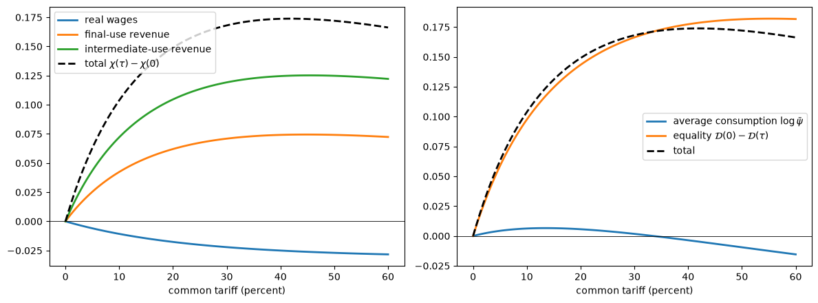
Fig. 72.1 Decompositions of worker welfare#
χ(5%) - χ(0) = 0.063; worker welfare peaks at 42 percent
A tariff lowers home’s real wages slightly, because it raises the price of imported goods and inputs and diverts production from home’s strongest sectors.
The rebates of tariff revenue more than make up for it over a wide range of tariffs, and revenue from imported inputs contributes more than revenue from imported final goods, because firms buy more imports than final users do.
Nearly all of the gain is in the equality term: an equal rebate is worth much more, in proportion, to a low-paid worker than to a high-paid one, while average consumption hardly changes.
These are the two findings that Bassetto et al. [2026] emphasize for the G7, where worker welfare rises by roughly \(0.05\) between free trade and a 5 percent tariff and peaks at about 40 percent.
The next figure shows how a rise in the tariff from 5 to 10 percent changes consumption in each sector, with sectors ordered by their workers’ baseline consumption.
change = 100 * (ψ[i_10] / ψ[i_5] - 1)
order = np.argsort(ψ[i_5])
fig, ax = plt.subplots(figsize=(8, 4))
ax.bar(range(len(order)), change[order], color='C0')
ax.set_xticks(range(len(order)))
ax.set_xticklabels([sectors[j].replace(' ', '\n', 1) for j in order])
ax.axhline(0, color='k', lw=0.6)
ax.set_ylabel("consumption change (percent)")
plt.tight_layout()
plt.show()
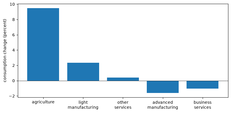
Fig. 72.2 Consumption changes by sector#
The three lowest-paid groups gain, by amounts that fall steeply with baseline consumption, and the two best-paid groups lose.
Bassetto et al. [2026] find the same pattern across quintiles of 30 sectors, with consumption rising by 4.3 percent in the lowest quintile and falling by 0.3 percent in the highest.
72.6. Dynamic tariff policy#
The dynamic analysis needs only \(\chi\), \(G\), and the parameters of Bassetto et al. [2026]: annual periods, \(\beta = 0.96\), \(\sigma = 0.5\), and \(\delta_k = 0.10\).
We collect them in a Policy tuple and define the objects of Institution Building Without Commitment in terms of
it.
Policy = namedtuple('Policy', ('χ', 'G', 'β', 'σ'))
β, σ, δ_k = 0.96, 0.5, 0.10

def make_policy(r_0, χ=χ_s, ρ=ρ_s):
    return Policy(χ=χ, G=lambda τ: 1 - δ_k + r_0 * ρ(τ), β=β, σ=σ)

def argmax(f, lo=0.0, hi=0.6):
    return minimize_scalar(lambda τ: -f(τ), bounds=(lo, hi), method='bounded',
                           options={'xatol': 1e-10}).x

def markov_tariff(pol):
    return argmax(lambda τ: pol.χ(τ) + pol.β / (1 - pol.β) * np.log(pol.G(τ)))

def best_constant_tariff(pol):
    return argmax(lambda τ: pol.χ(τ) + pol.β / (pol.σ * (1 - pol.β)) * np.log(pol.G(τ)))

def s_const(τ, pol):
    "The saving rate when the tariff is τ forever."
    return (pol.β * pol.G(τ)**(1 - pol.σ))**(1 / pol.σ)

def H(τ, s, pol):
    return pol.χ(τ) + pol.β / (1 - pol.β) * (np.log(s) + np.log(pol.G(τ)))

def growth_gap(r_0):
    "Long-run growth at the best constant tariff, minus 2 percent."
    pol = make_policy(r_0)
    τ_B = best_constant_tariff(pol)
    return s_const(τ_B, pol) * pol.G(τ_B) - 1.02

r_0 = brentq(growth_gap, 0.05, 0.5)
pol = make_policy(r_0)
τ_M, τ_B = markov_tariff(pol), best_constant_tariff(pol)
print(f"Markov tariff {100 * τ_M:.1f} percent, best constant tariff {100 * τ_B:.1f} percent")
print(f"growth at the Markov tariff {100 * (s_const(τ_M, pol) * pol.G(τ_M) - 1):.2f} percent")
Markov tariff 14.5 percent, best constant tariff 1.2 percent
growth at the Markov tariff 1.36 percent
fig, axes = plt.subplots(1, 2, figsize=(12, 4.5))
grid = np.linspace(0, 0.4, 201)
axes[0].plot(100 * grid, 100 * (pol.G(grid) - 1), lw=2)
axes[0].set_ylabel("net return to capital (percent a year)")
for weight, name in [(β / (1 - β), "Markov"), (β / (σ * (1 - β)), "best constant")]:
    objective = pol.χ(grid) + weight * np.log(pol.G(grid))
    axes[1].plot(100 * grid, objective - objective.max(), lw=2, label=f"{name} objective")
axes[1].set_ylabel("objective relative to its maximum")
for ax in axes:
    ax.axvline(100 * τ_B, color='C2', ls='--', lw=1, label=r"$\tau^B$")
    ax.axvline(100 * τ_M, color='C3', ls=':', lw=1.5, label=r"$\tau^M$")
    ax.set_xlabel("common tariff (percent)")
    ax.legend()
plt.tight_layout()
plt.show()
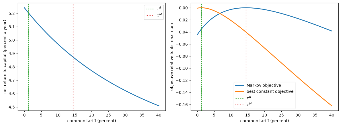
Fig. 72.3 Capital returns and tariff objectives#
The net return to capital falls from 5.2 percent a year at free trade to 4.5 percent at a 40 percent tariff.
The level at free trade is pinned down by the growth target, as it is in Bassetto et al. [2026], but the decline is an independent result, and it is close to the decline they report.
A Markov policymaker, who takes the current saving rate as given, weighs this fall against the static gain in \(\chi\) and chooses a tariff of 14.5 percent.
The best constant tariff puts \(1/\sigma = 2\) times as much weight on \(\log G\), and is only 1.2 percent.
72.6.1. When does a tariff pay?#
A first-order approximation at free trade explains why the model needs unequal wages to make tariffs attractive.
Write \(w_j = W_{1j}\) for the wage in home’s sector \(j\) and \(\bar w = \sum_j \lambda_j w_j\) for home’s average wage.
Suppose that world imports are a fraction \(x\) of world value added, and raise the common tariff from zero by \(d\tau\).
Tariff revenue rises by \(x \, d\tau\) times world value added.
If free trade is efficient, a small tariff changes world output only to second order, so this revenue comes out of factor incomes.
If, in addition, all factor prices fall in the same proportion, real wages and the real return to capital all fall by \(x \, d\tau\) in proportion.
Suppose that home imports the same fraction \(x\) of its own value added, and let \(\eta\) be labor’s share of home’s value added.
The rebate per home worker then rises by \(x \, d\tau / \eta\) times the average wage \(\bar w\), which is worth \(x \, d\tau \, \bar w / (\eta w_j)\) in proportion to a worker in sector \(j\).
Averaging logs over home’s workers gives
where \(\mathcal{I} \ge 1\) is the ratio of the average wage to its harmonic mean, which equals one only when all wages are equal.
A Markov policymaker raises the tariff above zero when \(d\chi + \frac{\beta}{1 - \beta} d \log G > 0\), and the best constant tariff is positive when the same holds with weight \(\frac{\beta}{\sigma(1 - \beta)}\):
Openness \(x\) has dropped out: what matters is how unequal consumption is across home’s workers, and how much of value added goes to them rather than to capital.
The next cell computes both sides of (72.3) at free trade.
free = solve_changes(tariff_wedges(0.0), model)
η = (model.α_l @ free['e'][0]) / ((model.α_l + model.α_k) @ free['e'][0])
w_0 = wages[0] / (λ @ wages[0])                   # relative wages at free trade
I = λ @ (1 / w_0)
r_free, G_free = pol.G(0) - 1 + δ_k, pol.G(0)
print(f"I = {I:.2f}, η = {η:.2f}, I / η = {I / η:.2f}")
print(f"thresholds: {1 + β / (1 - β) * r_free / G_free:.2f} for τ_M > 0, "
      f"{1 + β / (σ * (1 - β)) * r_free / G_free:.2f} for τ_B > 0")
I = 5.24, η = 0.57, I / η = 9.20
thresholds: 4.48 for τ_M > 0, 7.95 for τ_B > 0
With \(\beta = 0.96\), \(\sigma = 0.5\), \(\delta_k = 0.10\), and a 2 percent growth rate, a positive best constant tariff requires \(\mathcal{I}/\eta\) to exceed about 8, or \(\mathcal{I}\) to exceed about 4.5 when labor receives 57 percent of value added.
That is a lot of inequality: if all of home’s workers but a low-paid group earned the same wage, a group making up 40 percent of the labor force would need to earn a little less than a tenth of the average wage.
Our dual-economy calibration is built to satisfy (72.3), and Exercise 72.2 checks the approximation against exact solutions.
The same approximation suggests that the positive best constant tariff that Bassetto et al. [2026] find for the G7 rests on very unequal consumption across U.S. sectors at low tariffs, although they do not report a measure of that inequality.
72.6.2. Ramsey plan and plans sustained by Markov reversion#
We compute the Ramsey plan as in Institution Building Without Commitment, now over 80 years, with the tariff held constant afterward.
def saving_rates(τ, pol):
    "Saving rates for tariffs τ_0, ..., τ_N, with τ_N kept forever."
    s = np.empty(len(τ))
    s[-1] = s_const(τ[-1], pol)
    for t in range(len(τ) - 2, -1, -1):
        ratio = (pol.β * pol.G(τ[t + 1])**(1 - pol.σ))**(-1 / pol.σ) * (1 - s[t + 1])
        s[t] = 1 / (1 + ratio)
    return s

def action_payoffs(τ, pol):
    "Action payoffs V_0, ..., V_N for tariffs τ_0, ..., τ_N, with τ_N kept forever."
    s = saving_rates(τ, pol)
    V = np.empty(len(τ))
    V[-1] = H(τ[-1], s[-1], pol) / (1 - pol.β)
    for t in range(len(τ) - 2, -1, -1):
        V[t] = H(τ[t], s[t], pol) + pol.β * V[t + 1]
    return V

H_B = H(τ_B, s_const(τ_B, pol), pol)
V_markov = H(τ_M, s_const(τ_M, pol), pol) / (1 - β)
V_best = H_B / (1 - β)

horizon = 80
res = minimize(lambda τ: -action_payoffs(τ, pol)[0], np.full(horizon + 1, τ_B),
               bounds=[(0, 0.6)] * (horizon + 1), method='L-BFGS-B')
τ_R = res.x
V_R = action_payoffs(τ_R, pol)
print("Ramsey tariffs every 5 years (percent):", np.round(100 * τ_R[:35:5], 1))
print(f"first year of free trade: {np.argmax(τ_R < 1e-4)}")
print(f"smallest V_t - V_M along the Ramsey plan: {(V_R - V_markov).min():.3f}")
Ramsey tariffs every 5 years (percent): [14.5 11.5  8.7  6.3  4.1  2.1  0.3]
first year of free trade: 32
smallest V_t - V_M along the Ramsey plan: 0.993
The Ramsey plan starts at the Markov tariff, because the first tariff affects no saving decision, and then lowers the tariff by about a percentage point every two years, reaching free trade after 31 years.
Every continuation of the plan is worth more than the Markov equilibrium, so the plan is also the best plan sustained by the threat of permanent reversion to the Markov equilibrium, which Bassetto et al. [2026] call the best sustainable equilibrium.
72.6.3. Organizational equilibrium#
As in Institution Building Without Commitment, the organizational equilibrium keeps the action payoff constant at \(V^\ast = H^B / (1 - \beta)\), follows the transition map \(\tau_{t+1} = \mathcal{T}(\tau_t)\) implied by that requirement and the Euler equation, and starts at \(\tau_0 = \mathcal{T}(\tau^M)\), the lowest tariff that satisfies no delay.
def s_org(τ, H_B, pol):
    "The saving rate that keeps H(τ, s) equal to H_B."
    return np.exp((1 - pol.β) / pol.β * (H_B - pol.χ(τ)) - np.log(pol.G(τ)))

def transition(τ, τ_B, H_B, pol):
    "Next year's tariff on a path whose action payoff is constant at H_B / (1 - β)."
    if τ <= τ_B + 1e-8:
        return τ_B
    s = s_org(τ, H_B, pol)
    lhs = ((1 - s) / s)**(-pol.σ)
    f = lambda τ_next: (pol.β * pol.G(τ_next)**(1 - pol.σ)
                        * (1 - s_org(τ_next, H_B, pol))**(-pol.σ) - lhs)
    return brentq(f, τ_B, τ)                       # the root between τ_B and τ

𝒯 = lambda τ: transition(τ, τ_B, H_B, pol)

τ_O = [𝒯(τ_M)]
for t in range(1500):
    τ_O.append(𝒯(τ_O[-1]))
τ_O = np.array(τ_O)
V_O = action_payoffs(τ_O, pol)
print(f"max |V_t - V*| over the first 50 years = {np.abs(V_O[:50] - V_best).max():.1e}")
print("organizational tariffs (percent) in years 0, 10, 20, 50, 100:",
      np.round(100 * τ_O[[0, 10, 20, 50, 100]], 1))
max |V_t - V*| over the first 50 years = 8.8e-12
organizational tariffs (percent) in years 0, 10, 20, 50, 100: [11.8  7.9  6.6  4.8  3.7]
n_plot = 51
fig, axes = plt.subplots(1, 2, figsize=(12, 4.5))
grid_τ = np.linspace(τ_B, τ_M, 100)
axes[0].plot(100 * grid_τ, [100 * 𝒯(x) for x in grid_τ], 'C3', lw=2,
             label=r"$\mathcal{T}(\tau)$")
axes[0].plot(100 * grid_τ, 100 * grid_τ, 'k', lw=0.8, label="45-degree line")
axes[0].set_xlabel(r"current tariff $\tau_t$ (percent)")
axes[0].set_ylabel(r"next tariff $\tau_{t+1}$ (percent)")
axes[0].legend()
axes[1].plot(100 * τ_O[:n_plot], 'C3', lw=2, label="organizational equilibrium")
axes[1].plot(100 * τ_R[:n_plot], 'C0--', lw=2,
             label="Ramsey plan = best plan sustained by Markov reversion")
axes[1].plot(np.full(n_plot, 100 * τ_M), 'k:', lw=2, label="Markov equilibrium")
axes[1].set_xlabel("year")
axes[1].set_ylabel("tariff (percent)")
axes[1].legend(loc='center right')
plt.tight_layout()
plt.show()
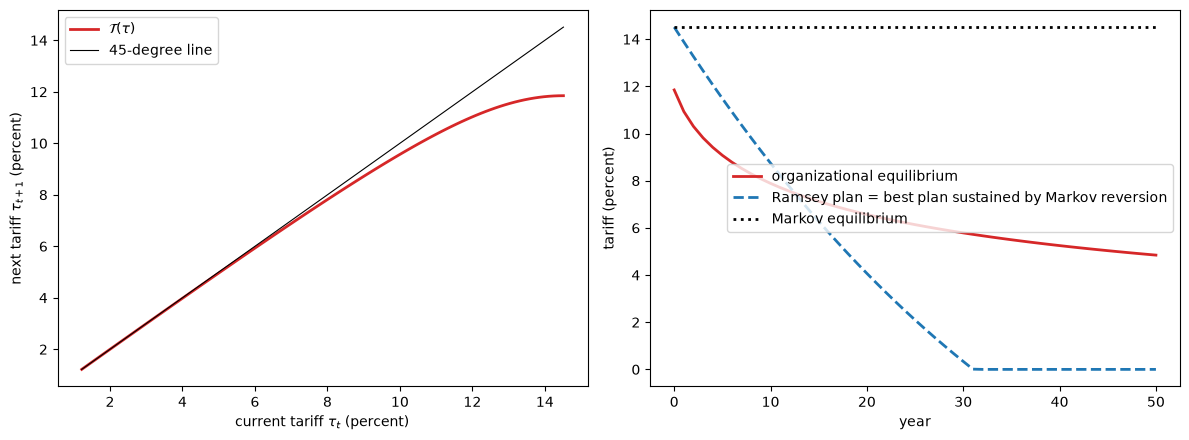
Fig. 72.4 Transition map and tariff paths#
The organizational equilibrium starts at 11.8 percent, below the Markov tariff, and liberalizes gradually: the tariff is 7.9 percent after 10 years and 4.8 percent after 50.
The transition map is flat at the Markov tariff and has slope one at \(\tau^B\), so liberalization slows as the tariff falls, and after a century the tariff is still 3.7 percent.
The Ramsey plan starts higher but liberalizes faster, as in the paths that Bassetto et al. [2026] compute for the G7.
72.6.4. A temporary protectionist shock#
Following Bassetto et al. [2026], suppose that in year 20 an unexpected shock sets the tariff to 10 percent.
t_shock, τ_shock = 20, 0.10
τ_O_shock = list(τ_O[:t_shock]) + [τ_shock]
while len(τ_O_shock) < n_plot:
    τ_O_shock.append(𝒯(τ_O_shock[-1]))
τ_R_shock = np.r_[τ_R[:t_shock], τ_shock, np.full(n_plot - t_shock - 1, τ_M)]
t_back = np.argmin(np.abs(τ_O - 𝒯(τ_shock)))
print(f"tariff after the shock: {100 * 𝒯(τ_shock):.1f} percent, close to the undisturbed "
      f"path's tariff in year {t_back}, a delay of about {t_shock + 1 - t_back} years")

fig, ax = plt.subplots(figsize=(8, 4.5))
ax.plot(100 * np.array(τ_O_shock), 'C3', lw=2, label="organizational equilibrium")
ax.plot(100 * τ_R_shock, 'C0--', lw=2, label="best plan sustained by Markov reversion")
ax.plot(np.full(n_plot, 100 * τ_M), 'k:', lw=2, label="Markov equilibrium")
ax.axvline(t_shock, color='gray', ls=':', lw=1)
ax.set_ylim(0, 16)
ax.set_xlabel("year")
ax.set_ylabel("tariff (percent)")
ax.legend(loc='lower right')
plt.show()
tariff after the shock: 9.6 percent, close to the undisturbed path's tariff in year 4, a delay of about 17 years
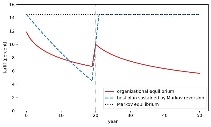
Fig. 72.5 Tariffs after a protectionist shock#
In year 21, the organizational equilibrium resumes from \(\mathcal{T}(0.10)\), close to the tariff that the undisturbed path reached in year 4, so the shock delays liberalization by about 17 years but leaves its destination unchanged.
The plan sustained by Markov reversion instead returns to the Markov tariff forever.
72.7. Trade blocs#
Bonadio et al. [2026] use a model of the same family to study the reorganization of world trade since 2015.
From changes in bilateral trade flows between 2015 and 2023, they infer changes in bilateral trade costs and classify countries as moving toward a U.S. bloc, toward a China bloc, or neither.
Trade costs rose between the two blocs but fell within them, and the ratio of world trade to world output did not fall: the world economy has been decoupling rather than deglobalizing.
Solving their production network model in changes, they find that the trade-cost changes raised real income in the median country by about 0.6 percent, and that many countries would have gained more by joining the other bloc, which suggests that motives other than trade are shaping the blocs.
Two features of their analysis bear on the questions of this lecture.
The trade-cost changes that they measure are bilateral, rising with some partners and falling with others, whereas the lead country of Bassetto et al. [2026] sets one tariff on all imports, which all other countries match.
Their comparison of 2015–2019 with 2015–2023 suggests that the fall in costs within blocs lagged the rise in costs between them, though the pandemic and the war in Ukraine offer another explanation.
Extending organizational equilibrium to several strategic countries, which a bloc structure calls for, requires generalizing the equilibrium concept, as Bassetto et al. [2026] note.
Exercise 72.3 takes a first step by asking how home’s Markov and best constant tariffs change when home and \(B\) tax only each other’s goods.
72.8. Connections to other lectures#
Institution Building Without Commitment defines organizational equilibrium and computes it in the growth model and the two-sector tariff model of Bassetto et al. [2024]; this lecture reuses its dynamic analysis unchanged.
Gradualism in Self-Enforcing Trade Agreements explains gradual liberalization by the incentive constraints of self-enforcing agreements between countries of different size [Bond and Park, 2002], rather than by the time inconsistency that drives the tariffs here.
72.9. Exercises#
Exercise 72.1
Suppose that home rebates tariff revenue in proportion to wages instead of equally per worker, so that a worker in sector \(j\) consumes \(W_{1j} (1 + T_1 / \sum_k W_{1k} L_{1k}) / P_1\).
The static equilibrium does not change, because the rebate rule changes neither total spending nor its composition.
Compute \(\chi(\tau)\) under this rule, and the Markov and best constant tariffs, holding \(r_0\) fixed.
Explain the result using (72.3).
Solution
χ_prop = (np.log(wages) @ λ + np.log(1 + (T_c + T_x) / (wages @ λ))
          - np.log(P_home))
pol_prop = make_policy(r_0, χ=CubicSpline(τ_grid, χ_prop))
print(f"χ(10%) - χ(0): equal rebate {χ_grid[i_10] - χ_grid[0]:.4f}, "
      f"proportional rebate {χ_prop[i_10] - χ_prop[0]:.4f}")
print(f"Markov tariff {100 * markov_tariff(pol_prop):.1f} percent, "
      f"best constant tariff {100 * best_constant_tariff(pol_prop):.1f} percent")
χ(10%) - χ(0): equal rebate 0.1038, proportional rebate 0.0136
Markov tariff 0.0 percent, best constant tariff 0.0 percent
A proportional rebate raises every worker’s consumption by the same proportion, so it does nothing for equality.
In (72.3), it replaces \(\mathcal{I}\) by one, and \(1/\eta \approx 1.76\) falls far short of both thresholds.
Both tariffs are zero: in this model, the motive for protection is redistribution through the equal rebate.
Exercise 72.2
Check the approximation (72.3).
Vary agriculture’s share of home’s employment from 0.25 to 0.46, scaling the other sectors’ shares proportionally and holding sectoral wage bills, and so the static equilibrium and \(r_0\), fixed.
For each value, compute \(\mathcal{I}/\eta\) and the Markov and best constant tariffs, and compare the values of \(\mathcal{I}/\eta\) at which the tariffs become positive with the thresholds in (72.3).
Solution
bills = wages * λ                       # sectoral wage bills, independent of λ
thresholds = [1 + β / (1 - β) * r_free / G_free,
              1 + β / (σ * (1 - β)) * r_free / G_free]
results = []
for λ_ag in np.linspace(0.25, 0.46, 22):
    λ_i = np.r_[λ_ag, λ[1:] * (1 - λ_ag) / λ[1:].sum()]
    w_i = bills / λ_i
    χ_i = np.log(w_i + (T_c + T_x)[:, None]) @ λ_i - np.log(P_home)
    pol_i = make_policy(r_0, χ=CubicSpline(τ_grid, χ_i))
    I_i = λ_i @ ((λ_i @ w_i[0]) / w_i[0])
    results.append((I_i / η, markov_tariff(pol_i), best_constant_tariff(pol_i)))
results = np.array(results)

fig, ax = plt.subplots()
ax.plot(results[:, 0], 100 * results[:, 1], 'o-', lw=2, label=r"Markov tariff $\tau^M$")
ax.plot(results[:, 0], 100 * results[:, 2], 's-', lw=2, label=r"best constant tariff $\tau^B$")
for value, style, name in zip(thresholds, [':', '--'], [r"$\tau^M$", r"$\tau^B$"]):
    ax.axvline(value, color='gray', ls=style, lw=1, label=f"approximate threshold for {name}")
ax.set_xlabel(r"$\mathcal{I} / \eta$")
ax.set_ylabel("tariff (percent)")
ax.legend()
plt.show()

for k, name in [(1, "Markov"), (2, "best constant")]:
    first = np.argmax(results[:, k] > 1e-4)
    print(f"{name} tariff first positive between I/η = {results[first - 1, 0]:.2f} "
          f"and {results[first, 0]:.2f}; threshold {thresholds[k - 1]:.2f}")
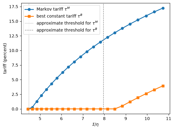
Markov tariff first positive between I/η = 4.44 and 4.64; threshold 4.48
best constant tariff first positive between I/η = 8.49 and 8.84; threshold 7.95
The vertical lines mark the two thresholds in (72.3).
The Markov tariff becomes positive almost exactly at its threshold, and the best constant tariff a little above its threshold, at \(\mathcal{I}/\eta\) between 8.5 and 8.8 rather than 7.95.
The approximation errs because our countries are not symmetric and wages do not all move in proportion, and the error matters more for the best constant tariff, whose larger weight on \(\log G\) magnifies any error in the return effect.
Beyond the thresholds, both tariffs rise steadily with inequality.
Exercise 72.3
Suppose that home and \(B\) impose the tariff \(\tau\) only on each other’s goods, while all other tariffs stay at the 5 percent baseline.
Write a function that returns these tariff wedges, solve the model on
τ_grid, and compute \(\chi(\tau)\) and \(\rho(\tau)\).Compute home’s Markov and best constant bilateral tariffs, holding \(r_0\) fixed, and compare them with the common tariffs.
How do the shares of \(A\) and \(B\) in home’s final spending change as the bilateral tariff rises from 5 to 30 percent?
Solution
def bilateral_wedges(τ, τ_0=0.05):
    D = tariff_wedges(τ_0)
    D[0, 2] = D[2, 0] = 1 + τ
    return D

w_b, T_b, P_b, ρ_b, from_A, from_B = [], [], [], [], [], []
start = None
for τ in τ_grid:
    eq = solve_changes(bilateral_wedges(τ), model, start)
    start = (eq['p'], eq['e'])
    w_b.append(model.α_l * eq['e'][0] / λ)
    T_b.append(eq['T_c'][0] + eq['T_x'][0])
    P_b.append(eq['P'][0])
    ρ_b.append(eq['κ'] / κ_0 / np.exp(model.μ @ np.log(eq['P'])))
    from_A.append(eq['πc'][1, 0] @ model.Φ)
    from_B.append(eq['πc'][2, 0] @ model.Φ)
w_b, T_b, P_b, ρ_b = map(np.array, (w_b, T_b, P_b, ρ_b))
χ_b = np.log(w_b + T_b[:, None]) @ λ - np.log(P_b)
pol_b = make_policy(r_0, χ=CubicSpline(τ_grid, χ_b), ρ=CubicSpline(τ_grid, ρ_b))

i_30 = np.argmin(np.abs(τ_grid - 0.30))
print(f"from 5 to 30 percent: Δχ bilateral {χ_b[i_30] - χ_b[i_5]:.3f}, common "
      f"{χ_grid[i_30] - χ_grid[i_5]:.3f}; Δ log ρ bilateral "
      f"{np.log(ρ_b[i_30] / ρ_b[i_5]):.4f}, common {np.log(ρ[i_30] / ρ[i_5]):.4f}")
print(f"bilateral tariffs: Markov {100 * markov_tariff(pol_b):.1f} percent, "
      f"best constant {100 * best_constant_tariff(pol_b):.1f} percent")
print(f"share of home's final spending from A: {100 * from_A[i_5]:.2f} -> "
      f"{100 * from_A[i_30]:.2f} percent; from B: {100 * from_B[i_5]:.2f} -> "
      f"{100 * from_B[i_30]:.2f} percent")
from 5 to 30 percent: Δχ bilateral 0.056, common 0.105; Δ log ρ bilateral -0.0122, common -0.0317
bilateral tariffs: Markov 20.4 percent, best constant 7.4 percent
share of home's final spending from A: 2.55 -> 2.73 percent; from B: 3.61 -> 2.30 percent
A bilateral tariff raises less revenue than a common one, so the gain in worker welfare is about half as large.
But it lowers the return to capital much less, about two-fifths as much, because it taxes only the trade between home and \(B\) and leaves most of world trade untouched.
Since the cost to capital accumulation falls by more than the gain to workers, both tariffs are higher than the corresponding common tariffs, and the best constant bilateral tariff is far from free trade.
Home’s final purchases from \(B\) fall by about a third, mostly in favor of home’s own goods; purchases from \(A\) rise only slightly.