55. A Competitive Entrepreneurial Model of a Stock Market#
55.1. Overview#
Two questions arise when we study the role of a stock market in an economy with production.
Is the allocation of risk and capital that results from competitive trading in firm shares and debt efficient in some appropriate sense?
What is, or should be, the objective of a firm?
The second question arises because profit maximization cannot be implemented when profits are uncertain and markets for contingent claims are incomplete, as they generally are when the only institution for trading risks is a market for firm shares.
Diamond [1967] showed that a stock market allocates risk and capital efficiently in a second-best sense, under a restriction on technology that Diamond called stochastic constant returns to scale.
That restriction also made stock market value maximization a sensible objective for a firm, one that, as Leland [1974] and Ekern and Wilson [1974] later showed, all shareholders agree on.
Kihlstrom and Laffont [1982] drop Diamond’s restriction on technology.
They replace the assumption that firms maximize their market value with the assumption that each firm is created and run by an entrepreneur who maximizes expected utility, choosing at the same time how to operate the firm, how to finance it, and which portfolio to hold.
Their economy is the one that Kihlstrom and Laffont [1979] had studied, with one addition: a stock market that lets entrepreneurs share the risks of their firms.
In the economy of Kihlstrom and Laffont [1979], which formalizes an idea of Knight [1921], individuals choose between running a risky firm and selling their resources for a safe return, and the less risk averse become entrepreneurs.
Kihlstrom and Laffont obtain a competitive model of a stock market by assuming
a continuum of individuals, in the manner of Aumann [1964], so that every trader takes all prices as given,
free entry: anyone can create a firm by paying a fixed set-up cost, and
a single random variable that affects the output of every firm, so that shares of firms that are run the same way are perfect substitutes.
Their main findings are
the Modigliani-Miller theorem and the proposition that a firm’s value equals the capital invested in it both follow from the absence of arbitrage opportunities, including arbitrage by creating a firm,
investors do not diversify: each holds shares only in firms run as the investor would run them,
these clienteles make the shareholders of each firm unanimous about how it should be run,
the equilibrium can be computed as the competitive equilibrium of a simple two-good exchange economy,
an equilibrium with classical price expectations, defined below, is efficient in Diamond’s second-best sense, though usually not in the first-best sense of Arrow and Debreu, and
the equilibrium reduces to Diamond’s when technology has stochastic constant returns to scale, and to the long-run competitive equilibrium with production at minimum average cost when there is no uncertainty.
This lecture sets out the model, computes its equilibrium in an example, and compares it with the equilibria of the same economy without a stock market and with complete markets.
It is closely related to Irrelevance of Capital Structures with Complete Markets and Equilibrium Capital Structures with Incomplete Markets, which study firms’ financial decisions and the Modigliani-Miller theorem in economies with complete and incomplete markets.
We use the following imports.
import numpy as np
import pandas as pd
import matplotlib.pyplot as plt
from collections import namedtuple
from scipy.optimize import minimize_scalar, brentq
55.2. The economy#
A continuum of individuals is indexed by \(\alpha \in [0, 1]\).
There are two goods: capital, which is only an input, and a consumption good that we call income.
Each individual begins with \(A > 0\) units of income and one unit of capital, and has a von Neumann-Morgenstern utility function \(u(\cdot, \alpha)\) of income, with \(u' > 0\) and \(u'' \le 0\).
Kihlstrom and Laffont’s Assumption A1 says that there are \(n\) types of individuals: all individuals of type \(i\) have the utility function \(u_i\), and the measure of type \(i\) is \(\mu_i > 0\), with \(\sum_i \mu_i = 1\).
Any individual can become an entrepreneur by spending its unit of capital as the set-up cost of a firm.
A firm that employs \(K\) units of operating capital, in addition to the unit of entrepreneurial capital, produces
units of income, where \(\tilde x\) is a random variable that takes values in a finite set \(X\) with probabilities \(p(x)\).
The same random variable \(\tilde x\) affects the output of every firm, and everyone agrees about its distribution.
The economy lasts one period: everybody decides whether to become an entrepreneur, firms choose their operating capital and how to finance it, and individuals trade capital, shares, and debt, all before \(\tilde x\) is realized; then output is produced and income is consumed.
The production function satisfies \(g(0, x) = 0\), \(g_K \ge 0\), and \(g_{KK} \le 0\), with strict inequalities whenever output is positive, and for each \(x\) at which output is positive there is a capital level \(K(x)\) at which
so that \(K(x)\) maximizes output per unit of capital, \(g(K, x) / (1 + K)\), and minimizes average cost, \(r (1 + K) / g(K, x)\), for any price \(r\) of capital.
An individual who does not become an entrepreneur is a capitalist: a capitalist can sell its unit of capital at the competitive price \(r\) or, when there is a stock market, use it to buy shares in firms.
Kihlstrom and Laffont allow \(x\) to be a vector, and in our example it has two elements, a productivity level \(z\) and a returns-to-scale parameter \(\theta\), with
If \(\theta\) were the same in every state, \(g\) would take the form \(h(K) z\), which is Diamond’s stochastic constant returns to scale, a case that we study below.
Letting \(\theta\) vary across states breaks that restriction: in states with positive output, (55.1) gives \(K(x) = \theta / (1 - \theta)\), so the scale at which capital is used most productively differs across states.
Our example has four states.
In the first, which has probability \(0.05\), every firm’s output is zero, because \(z = 0\).
The other three are equally likely, with \((z, \theta) \in \{(0.5, 0.2), (1, 0.5), (2, 0.8)\}\), so that decreasing returns set in early in the low-productivity state and late in the high-productivity one.
There are two types, a bold type with constant relative risk aversion \(0.5\) and a cautious type with relative risk aversion \(4\), which make up \(25\) and \(75\) percent of the population.
Every individual begins with \(A = 2\) units of income.
We describe each type’s preferences by a utility function and its derivative, the marginal utility.
Utility = namedtuple('Utility', ('u', 'du'))

def crra(ρ):
    "Constant relative risk aversion ρ; ρ = 0 is risk neutral."
    if ρ == 1:
        return Utility(u=np.log, du=lambda c: 1 / c)
    return Utility(u=lambda c: (c**(1 - ρ) - 1) / (1 - ρ),
                   du=lambda c: c**(-ρ))

Economy = namedtuple('Economy', ('z', 'θ', 'p', 'A', 'utilities', 'μ'))

def create_economy(z=(0.0, 0.5, 1.0, 2.0), θ=(0.5, 0.2, 0.5, 0.8),
                   p=(0.05, 0.95/3, 0.95/3, 0.95/3),
                   A=2.0, ρ=(0.5, 4.0), μ=(0.25, 0.75)):
    "Technology (z, θ, p), endowment A, and types (ρ, μ) of the example."
    return Economy(z=np.array(z), θ=np.array(θ), p=np.array(p), A=A,
                   utilities=[crra(ρ_i) for ρ_i in ρ], μ=np.array(μ))

def g(K, econ):
    "Output of a firm with operating capital K, one entry per state."
    return econ.z * K**econ.θ

def g_K(K, econ):
    "Marginal product of operating capital, one entry per state."
    return econ.θ * econ.z * K**(econ.θ - 1)

def output_per_capital(K, econ):
    "Output per unit of capital, g(K, x) / (1 + K), one entry per state."
    return g(K, econ) / (1 + K)

def K_star(econ):
    "The operating capital that maximizes expected output per unit of capital."
    return minimize_scalar(lambda K: -(econ.p @ output_per_capital(K, econ)),
                           bounds=(1e-8, 50), method='bounded',
                           options={'xatol': 1e-12}).x

econ = create_economy()
names = ['bold', 'cautious']
K_s = K_star(econ)
# maximal expected output per unit of capital
r_max = econ.p @ output_per_capital(K_s, econ)
positive = econ.z > 0
print(f"K(x) in the states with positive output: "
      f"{econ.θ[positive] / (1 - econ.θ[positive])}")
print(f"K* = {K_s:.3f}, E g(K*, x)/(1 + K*) = {r_max:.4f}, "
      f"E g_K(K*, x) = {econ.p @ g_K(K_s, econ):.4f}")
K(x) in the states with positive output: [0.25 1.   4.  ]
K* = 1.922, E g(K*, x)/(1 + K*) = 0.5776, E g_K(K*, x) = 0.5776
The capital level \(K^\ast\) maximizes expected output per unit of capital, and so, as the last two numbers confirm, it satisfies
We shall see that it is the scale at which a risk-neutral investor in a stock market economy wants a firm to operate, whatever the price of capital.
Fig. 55.1 shows output per unit of capital in the three states with positive output, and its expected value over all four states.
K_grid = np.linspace(0.01, 6, 400)
y_grid = output_per_capital(K_grid[:, None], econ)    # one column per state
fig, ax = plt.subplots(figsize=(9, 5))
for s in np.flatnonzero(positive):
    ax.plot(K_grid, y_grid[:, s], lw=2,
            label=rf'$z = {econ.z[s]:g}$, $\theta = {econ.θ[s]:g}$')
ax.plot(K_grid, y_grid @ econ.p, 'k--', lw=2, label='expected value')
ax.axvline(K_s, color='gray', ls=':', lw=1.5, label=r'$K^*$')
ax.set_xlabel('operating capital $K$')
ax.set_ylabel(r'$g(K, x) / (1 + K)$')
ax.legend(loc='upper left', bbox_to_anchor=(1.02, 1), frameon=False)
plt.tight_layout()
plt.show()
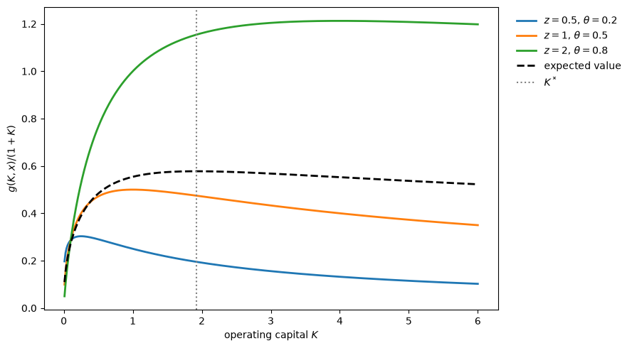
Fig. 55.1 Output per unit of capital#
55.3. Entrepreneurs without a stock market#
Kihlstrom and Laffont [1979] study this economy without a stock market.
They describe the alternative to entrepreneurship as working for a wage rather than selling capital at a price, but the structure is the same, and Section 5.8 of Kihlstrom and Laffont [1982] makes the comparison in the capital version that we use here.
An entrepreneur keeps all of its firm and buys the firm’s operating capital at the price \(r\), so its income is
A capitalist sells its unit of capital and receives the sure income \(A + r\).
An individual of type \(i\) becomes an entrepreneur if \(\max_K E u_i(A + g(K, \tilde x) - r K) > u_i(A + r)\) and a capitalist if the inequality is reversed.
As in Kihlstrom and Laffont [1979], we require that an entrepreneur can pay for its operating capital even if output is zero, \(K \le A / r\); this constraint does not bind in our example.
A type’s certainty-equivalent price \(r_i\) is the price of capital at which the type is indifferent between the two roles.
Because a more risk-averse individual values the random profit of a firm less, the more risk averse a type is, the lower is its certainty-equivalent price.
So less risk-averse types become entrepreneurs and more risk-averse types become capitalists, and the price of capital adjusts so that the demand for capital, one unit per firm plus its operating capital, equals the supply.
In the continuum of types that Kihlstrom and Laffont [1979] study, the equilibrium price is the certainty-equivalent price of a marginal type.
With finitely many types, it can also lie between the certainty-equivalent prices of two adjacent types; then every individual of the less risk averse of the two types, and of every type less risk averse than that, is an entrepreneur, and every other individual is a capitalist.
To compute the equilibrium, we use the “big \(K\), little \(k\)” device that is introduced in Rational Expectations Equilibrium and used in Investment Under Uncertainty and Cass-Koopmans Competitive Equilibrium.
Each individual is one of a continuum, so it takes the price of capital \(r\) as given, although \(r\) depends on what everybody does.
We first solve each individual’s problem, the choice of a role and of operating capital, at a given \(r\).
Only then do we impose that the individual choices are consistent with the market-wide price, by finding the \(r\) at which the demand for capital equals the supply.
In those lectures, little \(k\) (little \(y\) in Rational Expectations Equilibrium) is an individual’s choice and big \(K\) (big \(Y\)) is its economy-wide counterpart, which the individual takes as given.
Here the market-wide object is the price \(r\), and the letter \(K\), a firm’s operating capital, is an individual choice: a little \(k\) despite its capital letter.
def entrepreneur_K(r, ut, econ):
    "Operating capital chosen by an entrepreneur who keeps all of its firm."
    def f(K):
        return -(econ.p @ ut.u(econ.A + g(K, econ) - r * K))
    return minimize_scalar(f, bounds=(1e-8, econ.A / r), method='bounded',
                           options={'xatol': 1e-12}).x

def entrepreneur_value(r, ut, econ):
    "Expected utility of an entrepreneur who keeps all of its firm."
    K = entrepreneur_K(r, ut, econ)
    return econ.p @ ut.u(econ.A + g(K, econ) - r * K)

def ce_price(ut, econ):
    "The price of capital at which a type is indifferent between the two roles."
    return brentq(lambda r: entrepreneur_value(r, ut, econ) - ut.u(econ.A + r),
                  0.01, 5.0, xtol=1e-13)

def solve_no_stock_market(econ):
    """
    Price of capital and measures of entrepreneurs of each type in the economy
    without a stock market.  Types become entrepreneurs in order of their
    certainty-equivalent prices, least risk averse first.
    """
    n = len(econ.μ)
    # little k step, individual choices at a given r: a type prefers to be
    # an entrepreneur if r < r_ce, and an entrepreneur chooses operating
    # capital entrepreneur_K(r)
    r_ce = np.array([ce_price(ut, econ) for ut in econ.utilities])
    order = np.argsort(-r_ce)

    def demand(r, types):
        "Capital demanded at price r when all of the given types are firms."
        K = [entrepreneur_K(r, econ.utilities[t], econ) for t in types]
        return sum(econ.μ[t] * (1 + K_t) for t, K_t in zip(types, K))

    # big K step, market clearing: find the r at which demand equals supply
    for j_pos, j in enumerate(order):
        # is type j the marginal type, indifferent at its own price?
        r = r_ce[j]
        K_j = entrepreneur_K(r, econ.utilities[j], econ)
        n_j = (1 - demand(r, order[:j_pos])) / (1 + K_j)
        if 0 <= n_j <= econ.μ[j]:
            entrepreneurs = np.zeros(n)
            entrepreneurs[order[:j_pos]] = econ.μ[order[:j_pos]]
            entrepreneurs[j] = n_j
            return r, entrepreneurs, r_ce
        # otherwise, does the price lie between two adjacent r_ce?
        if j_pos + 1 < n:
            f = lambda r: demand(r, order[:j_pos + 1]) - 1
            r_next = r_ce[order[j_pos + 1]]
            if f(r_next) * f(r) < 0:
                entrepreneurs = np.zeros(n)
                entrepreneurs[order[:j_pos + 1]] = econ.μ[order[:j_pos + 1]]
                return brentq(f, r_next, r), entrepreneurs, r_ce
    raise RuntimeError("no equilibrium found")

r_ns, entrepreneurs_ns, r_ce = solve_no_stock_market(econ)
print(f"certainty-equivalent prices: "
      f"bold {r_ce[0]:.4f}, cautious {r_ce[1]:.4f}")
print(f"equilibrium price of capital r = {r_ns:.4f}")
for i, (name, ut) in enumerate(zip(names, econ.utilities)):
    print(f"{name:9s}: measure of entrepreneurs "
          f"{entrepreneurs_ns[i]:.3f} of {econ.μ[i]:.2f}, "
          f"operating capital {entrepreneur_K(r_ns, ut, econ):.3f}")
certainty-equivalent prices: bold 0.5401, cautious 0.4260
equilibrium price of capital r = 0.4260
bold     : measure of entrepreneurs 0.250 of 0.25, operating capital 2.283
cautious : measure of entrepreneurs 0.111 of 0.75, operating capital 0.621
All bold individuals become entrepreneurs, and the cautious type is the marginal type: some cautious individuals are entrepreneurs and the rest are capitalists, so the price of capital equals the cautious type’s certainty-equivalent price.
Bold individuals strictly prefer to be entrepreneurs: their certainty-equivalent income is about \(2.75\), against \(2.43\) for a capitalist, while with a stock market, as we shall see, everybody is indifferent between the two roles.
The bold entrepreneurs run much larger firms than the cautious ones.
Kihlstrom and Laffont [1979] show that less risk-averse entrepreneurs run larger firms when the states can be ordered so that a better state raises both output and the marginal product of capital; in our example, with the states ordered as listed, this holds for \(K\) above about \(0.1\), a range that includes every firm size in our equilibria.
The next cell shows incomes state by state.
print(f"{'capitalist':22s}: {econ.A + r_ns:.3f} in every state")
for name, ut in zip(names, econ.utilities):
    K = entrepreneur_K(r_ns, ut, econ)
    c = econ.A + g(K, econ) - r_ns * K
    print(f"{name + ' entrepreneur':22s}: {np.round(c, 3)}")
capitalist            : 2.426 in every state
bold entrepreneur     : [1.027 1.617 2.538 4.898]
cautious entrepreneur : [1.736 2.19  2.523 3.101]
Entrepreneurs bear all of the risk of their firms, and capitalists bear none.
Kihlstrom and Laffont [1979] show that the equilibrium is inefficient in three ways.
Only entrepreneurs bear risk, and risk-averse entrepreneurs cannot share it.
Firms run by entrepreneurs with different attitudes toward risk operate at different scales, though, with a concave technology hit by a common shock, total output in every state would be larger if capital were spread evenly across firms.
The number of firms is too large or too small.
All three inefficiencies stem from the absence of opportunities to trade risk: the equilibrium is efficient if entrepreneurs are risk neutral, and it is efficient in a restricted sense that takes the absence of risk sharing as given.
The obvious remedy is a stock market.
55.4. Adding a stock market#
55.4.1. Financing a firm#
Now an entrepreneur \(\alpha\) who employs operating capital \(K(\alpha)\) can also sell shares in its firm, retaining a fraction \(\gamma(\alpha)\) of them.
A share sells at a competitive price \(M(\alpha)\) in units of capital.
If the entrepreneur also borrows \(B(\alpha)\) units of capital, repaying \(r B(\alpha)\) units of income, the firm’s profits are
and the entrepreneur’s income is
The term in braces is the capital that the entrepreneur raises by selling shares, less the part of the firm’s operating capital that is not financed by debt; the entrepreneur sells this net amount of capital at the price \(r\), or buys it if it is negative.
More generally, an entrepreneur or a capitalist can hold a portfolio of shares in many firms, short sales are not allowed, and incomes may not be negative in any state.
Two firms with the same operating capital \(K\) and debt \(B\) have identical profits in every state, so Kihlstrom and Laffont assume that, in equilibrium, a single function \(N(K, B)\) gives the price of a share in any firm that chooses \((K, B)\), so that \(M(\alpha) = N(K(\alpha), B(\alpha))\).
55.4.2. Equilibrium#
A competitive stock market entrepreneurial equilibrium consists of a division of individuals into entrepreneurs and capitalists, a price \(r\) of capital, a share price function \(N\), operating and financial decisions \((K, B)\) for every firm, and a portfolio for every individual, such that
every entrepreneur chooses \((K, B)\) and a portfolio to maximize expected utility, taking \(r\) and \(N\) as given and recognizing that the price of its own firm’s shares is \(N(K, B)\),
every capitalist chooses a portfolio to maximize expected utility,
nobody would rather switch roles, and
the supply of shares in every firm equals the demand, and the supply of capital equals the demand.
Entrepreneurs are price takers: an entrepreneur takes the function \(N\) as given, just as a competitive firm takes the price of its output as given.
This is the “big \(K\), little \(k\)” device again, with the price function \(N\) joining \(r\) as a market-wide object that each individual takes as given.
Because \(N\) is a function, an entrepreneur takes as given the price that its shares would fetch at any \((K, B)\), including choices that no firm makes, and Exercise 55.4 shows that these off-equilibrium prices can change the equilibrium.
Equilibrium Capital Structures with Incomplete Markets uses the same version of the device, in which a firm takes as given price functions defined at every choice of capital and debt.
55.5. Free entry and the Modigliani-Miller theorem#
A firm that employs \(K\) units of operating capital, \(B\) of them financed with debt, uses \(1 + K - B\) units of its owner’s capital.
Kihlstrom and Laffont call the share price function
and the corresponding price expectations classical: at these prices a firm is worth exactly the capital invested in it.
Proposition 1 of Kihlstrom and Laffont [1982] states that in any equilibrium \(N(K, B) \le N_c(K, B)\) for every \((K, B)\), not only for the choices that firms actually make.
The argument is an arbitrage argument.
Compare a capitalist who holds some portfolio with an individual who creates a firm that chooses \((K, B)\), sells all of its shares at the price \(N(K, B)\), and buys the same portfolio.
The second individual gives up its unit of capital, receives \(N(K, B)\) units from selling shares, and pays \(K - B\) units for operating capital not financed by debt, as in (55.3) with \(\gamma = 0\), so that in every state its income \(W_E\) and the capitalist’s income \(W_C\) differ by
If \(N(K, B) > N_c(K, B)\) at some \((K, B)\), then creating a firm and selling it would raise every capitalist’s income in every state, so everybody would become an entrepreneur, and nobody would be left to supply operating capital.
Proposition 2 states that at the choices \((K, B)\) that firms actually make, \(N(K, B) = N_c(K, B)\), so that every individual is indifferent between being an entrepreneur and being a capitalist.
If a firm sold for less than the capital invested in it, its entrepreneur would do better by becoming a capitalist and buying the same portfolio.
Assumption A1 is needed here.
If an entrepreneur were the only individual who wanted a firm run its way, then by becoming a capitalist it would remove an investment opportunity that nobody else would provide, and the arbitrage argument would fail.
Because every type has positive measure, no individual is unique in this sense, and the argument goes through.
When \(N = N_c\), the value of a firm, its share price plus its debt, is \(N(K, B) + B = 1 + K\), which does not depend on how the firm is financed.
That is the Modigliani-Miller theorem [Modigliani and Miller, 1958].
Substituting \(N = N_c\) into the incomes of entrepreneurs and capitalists shows that both equal
where \(\Gamma(d\beta)\) is the number of shares that the individual holds in firms \(\beta\).
Debt \(B\) has disappeared, so nobody cares how any firm is financed, and the role of entrepreneur offers nothing that being a capitalist does not.
The equilibrium price function \(N\) is pinned down only for the \((K, B)\) that firms actually choose.
For other choices, \(N(K, B)\) is an expectation about the price of a firm that nobody creates, which can never be confirmed or refuted by observed trades.
Free entry implies only the upper bound of Proposition 1, so there can be other equilibria, with \(N < N_c\) at choices that no firm makes, and Section 5.7 of Kihlstrom and Laffont [1982] conjectures that such equilibria exist and are, in general, inefficient; Exercise 55.4 constructs some of them in our example.
Kihlstrom and Laffont focus on equilibria with classical expectations, \(N = N_c\) everywhere, which they justify by a strong form of rational expectations: \(N_c\) is the only price function that could be confirmed at every \((K, B)\).
Requiring confirmation at every \((K, B)\), and not only at the choices that firms make, resembles the requirement in Rational Expectations Equilibrium that the perceived law of motion equal the actual law of motion as a whole function, and not only along the equilibrium path.
The analogy is imperfect in one respect: here, beliefs about prices at choices that no firm makes affect what entrepreneurs choose.
Kihlstrom and Laffont’s weaker requirement, confirmation only at the choices that firms make, is the logic of a self-confirming equilibrium [Fudenberg and Levine, 1993], as in Self-Confirming Equilibria: beliefs about the consequences of actions that nobody takes are never tested, so they need not equal \(N_c\).
This is the issue that Bisin et al. [2018] address with rational conjectures about prices in regions of the state space that are not visited in equilibrium, as described in Equilibrium Capital Structures with Incomplete Markets.
From now on, we assume that \(N = N_c\).
55.6. No gains from diversification#
Because every firm’s output depends on the same \(\tilde x\) and \(g\) is concave in \(K\), a diversified portfolio is dominated by a stake in a single firm.
Suppose that a portfolio holds \(S = \int \Gamma(d\beta)\) shares in total, in firms whose average operating capital is \(\bar K = \int K(\beta) \, \Gamma(d\beta) / S\).
Jensen’s inequality gives, in every state \(x\),
By (55.4), holding \(S\) shares of a firm that employs \(\bar K\) costs the same as the portfolio, and it pays at least as much in every state.
So, by Proposition 3 of Kihlstrom and Laffont [1982], every entrepreneur holds shares only in its own firm and in firms run the same way, and every capitalist holds shares only in firms run as it would run them.
Newbery [1977] had obtained the same mathematical result, with an interpretation in terms of sharecropping.
The next cell checks the inequality for a portfolio split equally between two firms.
K_1, K_2 = 0.5, 3.0
diversified = 0.5 * g(K_1, econ) + 0.5 * g(K_2, econ)
undiversified = g(0.5 * K_1 + 0.5 * K_2, econ)
print("diversified portfolio  :", np.round(diversified, 4))
print("single firm at mean K  :", np.round(undiversified, 4))
diversified portfolio  : [0.     0.5291 1.2196 2.9826]
single firm at mean K  : [0.     0.5592 1.3229 3.1294]
The single firm pays at least as much in every state, and more in every state with positive output.
The argument depends on the common random variable: if firms’ outputs were independent, holding shares in many firms would reduce risk, and investors would diversify.
55.7. Clienteles and a two-good exchange economy#
An investor who holds \(\gamma\) shares in firms that employ \(K\) units of operating capital has income
Kihlstrom and Laffont assume that there is a state in which every firm’s output is zero, like the first state of our example, so that ruling out negative income requires \(A + r [1 - \gamma(1 + K)] \ge 0\).
An entrepreneur of type \(i\) chooses \((K, \gamma)\) to maximize the expected utility of this income, and a capitalist of type \(i\) chooses \(\gamma\) given the \(K\) that it would choose as an entrepreneur.
So all firms owned by type \(i\) investors operate at the same level \(K_i\), and their shareholders unanimously approve of it.
This clientele effect, which Proposition 4 of Kihlstrom and Laffont [1982] formalizes, delivers unanimity within each firm without any restriction on technology.
There are \(\nu_i = \gamma_i \mu_i\) firms of type \(i\), and the market for capital clears when
Since everyone is indifferent between the two roles, any \(\nu_i\) of the type \(i\) individuals can be the entrepreneurs; if \(\gamma_i > 1\), there are more type \(i\) firms than type \(i\) individuals, and individuals of other types set up the extra firms, run them as type \(i\) would, and sell all of their shares.
To compute an equilibrium, Kihlstrom and Laffont define the equity capital that a type \(i\) investor supplies to firms,
so that the investor holds \(\gamma_i = C_i / (1 + K_i)\) shares, a number that can exceed one, and has income \(A + r (1 - C_i) + C_i \, g(K_i, \tilde x) / (1 + K_i)\).
A type \(i\) investor then solves
In this problem each unit of equity capital earns the random return \(g(K, \tilde x)/(1 + K)\), output per unit of capital, and the investor chooses both how much equity capital to supply and how the firms that receive it should operate.
Kihlstrom and Laffont call the resulting equilibrium a capital management equilibrium, because without uncertainty a firm run this way would maximize output per unit of capital, as labor-managed firms maximize output per worker.
\(F^i\) is not concave in \((K, C)\) jointly, because \(C\) multiplies a function of \(K\).
But Lemma 2 of Kihlstrom and Laffont [1982] shows that, when \(u_i\) is strictly concave, the investor’s problem has at most one solution with \(K > 0\), and Lemma 3 shows that, for each \(C\), a unique \(K_i(C)\) maximizes \(F^i(K, C)\).
So we can solve (55.6) by a nested search: for each \(C\), find \(K_i(C)\), and then search over \(C\).
The equilibrium is the competitive equilibrium of a two-good exchange economy, with goods \(G\) (income) and \(C\) (equity capital), prices \(1\) and \(r\), an endowment \((A, 1)\) for everyone, and preferences
Every individual faces the budget constraint \(G = A + r (1 - C)\), and the market for equity capital clears when \(\sum_i \mu_i C_i = 1\), which is (55.5).
This reduction lets Kihlstrom and Laffont prove that an equilibrium exists by standard arguments, and it lets us compute one: we solve each type’s problem (55.6) for a given \(r\), and adjust \(r\) until the market for equity capital clears.
def best_K(G, C, ut, econ):
    "The operating capital that maximizes E u(G + C g(K, x)/(1 + K))."
    f = lambda K: -(econ.p @ ut.u(G + C * output_per_capital(K, econ)))
    return minimize_scalar(f, bounds=(1e-8, 50), method='bounded',
                           options={'xatol': 1e-12}).x

def V(G, C, ut, econ):
    "Expected utility from safe income G and equity capital C, at best_K."
    K = best_K(G, C, ut, econ)
    return econ.p @ ut.u(G + C * output_per_capital(K, econ))

def solve_investor(r, ut, econ):
    "The (K, C) that maximizes F(K, C) subject to the bankruptcy constraint."
    # little k step: one type's choices, taking the price r as given
    C = minimize_scalar(lambda C: -V(econ.A + r * (1 - C), C, ut, econ),
                        bounds=(0, econ.A / r + 1), method='bounded',
                        options={'xatol': 1e-12}).x
    return best_K(econ.A + r * (1 - C), C, ut, econ), C

def equity_demand(r, econ):
    "Total demand for equity capital, sum of μ_i C_i, at the price r."
    return sum(μ_i * solve_investor(r, ut, econ)[1]
               for μ_i, ut in zip(econ.μ, econ.utilities))

def solve_stock_market(econ):
    "Price of capital and each type's (K, C) when all types are risk averse."
    r_max = econ.p @ output_per_capital(K_star(econ), econ)
    # big K step: find the r at which the types' choices clear the market
    r = brentq(lambda r: equity_demand(r, econ) - 1,
               0.05 * r_max, (1 - 1e-6) * r_max, xtol=1e-13)
    return r, [solve_investor(r, ut, econ) for ut in econ.utilities]

def incomes(K, C, r, econ):
    "An investor's income in each state, given (K, C) and the price r."
    return econ.A + r * (1 - C) + C * output_per_capital(K, econ)

r_sm, solutions = solve_stock_market(econ)
print(f"price of capital r = {r_sm:.4f}  (E g(K*, x)/(1 + K*) = {r_max:.4f})")
print(f"bankruptcy bound on C: {econ.A / r_sm + 1:.3f}")
for i, (K, C) in enumerate(solutions):
    γ = C / (1 + K)
    print(f"{names[i]:9s}: K = {K:.4f}, C = {C:.3f}, γ = {γ:.3f}, "
          f"firms ν = {γ * econ.μ[i]:.3f}, income when output is zero = "
          f"{econ.A + r_sm * (1 - C):.3f}")
price of capital r = 0.4948  (E g(K*, x)/(1 + K*) = 0.5776)
bankruptcy bound on C: 5.042
bold     : K = 1.5661, C = 2.932, γ = 1.143, firms ν = 0.286, income when output is zero = 1.044
cautious : K = 1.5348, C = 0.356, γ = 0.140, firms ν = 0.105, income when output is zero = 2.319
Both types run firms that are smaller than the risk-neutral scale \(K^\ast\).
Valuing income by its marginal utility, they give less weight than its probability to the high-productivity state, the only state in which output per unit of capital is still rising at \(K^\ast\), and more weight to the low-productivity state, in which decreasing returns set in early.
The bold type supplies almost three units of equity capital per person, buying capital from the cautious type, which supplies only about a third of its unit and sells the rest.
Since \(\gamma > 1\) for the bold type, there are more bold-type firms than bold individuals, and some cautious individuals set up firms, run them as the bold type would, and sell all of their shares.
Neither type’s bankruptcy constraint binds.
With constant relative risk aversion, marginal utility becomes infinite as income falls to zero, so no type would choose to have zero income in the state in which output is zero.
The two types choose slightly different operating capital, so shareholders of different firms disagree, though every firm’s own shareholders agree.
Fig. 55.2 shows the solution \(K_i(C)\) of each type’s problem for a given \(C\), at the equilibrium price of capital.
As \(C\) shrinks to zero, the investor’s income becomes riskless, and \(K_i(C)\) approaches the risk-neutral scale \(K^\ast\), which is Lemma 3 of Kihlstrom and Laffont [1982].
C_grid = np.linspace(0.01, 4.5, 60)
fig, ax = plt.subplots(figsize=(8, 5))
for i, ut in enumerate(econ.utilities):
    K_of_C = [best_K(econ.A + r_sm * (1 - C), C, ut, econ) for C in C_grid]
    ax.plot(C_grid, K_of_C, lw=2, label=names[i])
    K_i, C_i = solutions[i]
    ax.plot(C_i, K_i, 'ko', label='equilibrium' if i == 0 else None)
ax.axhline(K_s, color='gray', ls=':', lw=1.5, label=r'$K^*$')
ax.set_xlabel('equity capital $C$')
ax.set_ylabel('operating capital $K_i(C)$')
ax.legend()
plt.show()
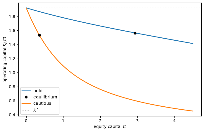
Fig. 55.2 Operating capital for given equity capital#
The dots mark the equilibrium choices.
Fig. 55.3 shows the market for equity capital: the total demand \(\sum_i \mu_i C_i(r)\) falls as the price of capital rises, and it equals the supply of one unit at the equilibrium price.
r_grid = np.linspace(0.35, 0.999 * r_max, 40)
fig, ax = plt.subplots(figsize=(8, 5))
ax.plot(r_grid, [equity_demand(r, econ) for r in r_grid], lw=2,
        label='demand for equity capital')
ax.axhline(1, color='k', lw=1, label='supply')
ax.axvline(r_max, color='gray', ls=':', lw=1.5,
           label=r'$E\,g(K^*, x) / (1 + K^*)$')
ax.plot(r_sm, 1, 'ko')
ax.set_xlabel('price of capital $r$')
ax.set_ylabel('equity capital')
ax.legend()
plt.show()
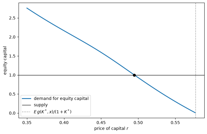
Fig. 55.3 The market for equity capital#
55.7.1. The price of capital#
The first-order conditions of (55.6) with respect to \(K\) and \(C\) give the price of capital in Theorem 1 of Kihlstrom and Laffont [1982].
Let \(c_i(x)\) be the income of type \(i\) in state \(x\), and let \(m_i(x) = u_i'(c_i(x)) / E u_i'(c_i(\tilde x))\) be its stochastic discount factor.
Then, for every risk-averse type whose bankruptcy constraint does not bind,
So the price of capital is the value of its marginal product and also the value of output per unit of capital, both valued with the type’s stochastic discount factor.
Because the return to equity capital is high in states in which investors’ marginal utility is low, its value is below its expected value: with risk-averse investors, the price of capital is below expected output per unit of capital.
The next cell checks (55.7) for both types.
def sdf(K, C, r, ut, econ):
    "A type's stochastic discount factor m(x)."
    marg_u = ut.du(incomes(K, C, r, econ))
    return marg_u / (econ.p @ marg_u)

for i, (K, C) in enumerate(solutions):
    m = sdf(K, C, r_sm, econ.utilities[i], econ)
    print(f"{names[i]:9s}: E[m g_K] = {econ.p @ (m * g_K(K, econ)):.5f}, "
          f"E[m g/(1+K)] = {econ.p @ (m * output_per_capital(K, econ)):.5f}, "
          f"E g/(1+K) = {econ.p @ output_per_capital(K, econ):.5f}")
bold     : E[m g_K] = 0.49477, E[m g/(1+K)] = 0.49477, E g/(1+K) = 0.57528
cautious : E[m g_K] = 0.49477, E[m g/(1+K)] = 0.49477, E g/(1+K) = 0.57481
55.7.2. Why do the clienteles nearly agree?#
The two types’ operating capital differs by only about 2 percent, though the cautious type’s relative risk aversion is eight times the bold type’s.
A mean-variance approximation explains why.
Write \(y(K, x) = g(K, x) / (1 + K)\) for output per unit of capital and \(y_K\) for its derivative with respect to \(K\), so that type \(i\)’s income is \(c_i = A + r (1 - C_i) + C_i \, y(K_i, \tilde x)\).
A first-order expansion of marginal utility around expected income gives
where \(a_i = -u_i'' / u_i'\) is the type’s absolute risk aversion, so that \(b_i = \rho_i C_i / E c_i\) for constant relative risk aversion \(\rho_i\).
The first-order conditions of (55.6) with respect to \(C\) and \(K\) are \(E[m_i (y - r)] = 0\) and \(E[m_i \, y_K] = 0\).
Substituting the approximation gives
and eliminating \(b_i\) leaves
one equation in \(K\) that does not involve preferences.
So, to this order of approximation, every type chooses the same \(K\), and a type’s risk aversion determines only how much equity capital it supplies: a more risk-averse type supplies less, so that \(b_i\) is the same for every type.
Differences in operating capital come from the next term of the expansion, \(\tfrac12 (u_i'''/u_i') \, C_i^2 \, (y - E y)^2\), which brings in third moments such as \(\operatorname{Cov}((y - E y)^2, y_K)\).
Because \(C_i = b_i / a_i\), the weight on this term is \(\tfrac12 b_i^2 \, u_i''' u_i' / (u_i'')^2\), which, for a given \(b_i\), is proportional to the ratio of prudence \(-u_i'''/u_i''\) to absolute risk aversion; with constant relative risk aversion the ratio is \((\rho_i + 1)/\rho_i\), which is \(3\) for the bold type and \(1.25\) for the cautious type.
That is why, in the next cell, the bold type’s operating capital is further from the mean-variance value than the cautious type’s.
The next cell solves the preference-free equation at the equilibrium price of capital and compares each type’s \(b_i\) with \((E y - r) / \operatorname{Var}(y)\).
def y_K(K, econ):
    "Derivative of output per unit of capital with respect to K."
    return g_K(K, econ) / (1 + K) - g(K, econ) / (1 + K)**2

def mean_variance_condition(K, r, econ):
    "E y_K Var(y) - (E y - r) Cov(y, y_K), whose root is the common K."
    y, dy = output_per_capital(K, econ), y_K(K, econ)
    Ey, Edy = econ.p @ y, econ.p @ dy
    var, cov = econ.p @ (y - Ey)**2, econ.p @ ((y - Ey) * (dy - Edy))
    return Edy * var - (Ey - r) * cov

def absolute_risk_aversion(ut, c, h=1e-6):
    "-u''(c)/u'(c), with u'' computed by a central difference."
    return -(ut.du(c + h) - ut.du(c - h)) / (2 * h) / ut.du(c)

K_mv = brentq(mean_variance_condition, 0.3, K_s, args=(r_sm, econ))
print(f"mean-variance approximation: K = {K_mv:.4f} for every type")
for i, (K, C) in enumerate(solutions):
    y = output_per_capital(K, econ)
    var = econ.p @ (y - econ.p @ y)**2
    mean_income = econ.p @ incomes(K, C, r_sm, econ)
    b_i = absolute_risk_aversion(econ.utilities[i], mean_income) * C
    print(f"{names[i]:9s}: K = {K:.4f}, b_i = {b_i:.3f}, "
          f"(E y - r)/Var(y) = {(econ.p @ y - r_sm) / var:.3f}")
mean-variance approximation: K = 1.5199 for every type
bold     : K = 1.5661, b_i = 0.537, (E y - r)/Var(y) = 0.526
cautious : K = 1.5348, b_i = 0.564, (E y - r)/Var(y) = 0.530
The approximation puts both types’ operating capital within about 3 percent of their actual choices, and it gets their \(b_i\) roughly right.
Fig. 55.4 shows the argument at a glance: the two types’ curves \(K_i(C)\) look different when plotted against \(C\) in Fig. 55.2, but plotted against \(b_i\) they nearly coincide.
def K_and_b(C, r, ut, econ):
    "A type's K_i(C) and its b = a_i(E c) C at the price r."
    K = best_K(econ.A + r * (1 - C), C, ut, econ)
    mean_income = econ.p @ incomes(K, C, r, econ)
    return K, absolute_risk_aversion(ut, mean_income) * C

fig, ax = plt.subplots(figsize=(8, 5))
for i, ut in enumerate(econ.utilities):
    K_vals, b_vals = np.array([K_and_b(C, r_sm, ut, econ)
                               for C in C_grid]).T
    ax.plot(b_vals, K_vals, lw=2, label=names[i])
    K_i, b_i = K_and_b(solutions[i][1], r_sm, ut, econ)
    ax.plot(b_i, K_i, 'ko', label='equilibrium' if i == 0 else None)
ax.axhline(K_s, color='gray', ls=':', lw=1.5, label=r'$K^*$')
ax.set_xlim(0, 2)
ax.set_xlabel(r'$b_i = a_i(E\,c_i) \, C$')
ax.set_ylabel('operating capital $K_i(C)$')
ax.legend()
plt.show()
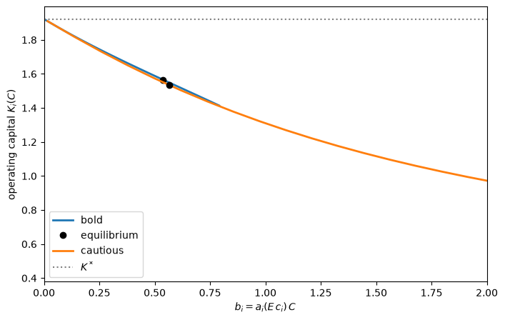
Fig. 55.4 Operating capital and the coefficient \(b_i\)#
Because the two types also choose nearly the same \(b_i\), their equilibrium points nearly coincide.
With quadratic utility, marginal utility is linear in income, so the approximation is exact, and every type chooses exactly the same \(K\), provided that the preference-free equation has a single root in the relevant range; this is an instance of the aggregation results of Rubinstein [1974], and Exercise 55.2 asks you to verify it.
55.8. Efficiency#
55.8.1. Diamond’s second-best efficiency#
Diamond [1967] proposed judging a stock market economy against the allocations that a planner could achieve with the same institutions.
Kihlstrom and Laffont adapt Diamond’s concept to their economy: the planner can decide who becomes an entrepreneur, how much capital each firm receives, and which shares and safe payments each individual gets, but cannot give anybody a payment that depends on the state other than through shares of firms’ output.
Theorem 2 of Kihlstrom and Laffont [1982] states that an equilibrium with \(N = N_c\) is efficient in this restricted sense: no allocation that uses only the stock market’s institutions makes some individuals better off and nobody worse off.
The proof combines Proposition 3, which shows that allocations with diversified portfolios are dominated, with the efficiency of competitive equilibria in the two-good exchange economy.
This extends Diamond’s efficiency result from technologies with stochastic constant returns to scale to any concave technology, at the cost of assuming free entry.
We can check Theorem 2 in our example.
By Proposition 3, a planner restricted to the stock market’s institutions can do no better than give each individual of type \(i\) a safe income \(G_i\) and equity capital \(C_i\) in firms that all operate at the same scale, and the best scale for that individual gives it expected utility \(V^i(G_i, C_i)\).
The planner’s resource constraints are \(\sum_i \mu_i G_i = A\) and \(\sum_i \mu_i C_i = 1\).
Treating individuals of a type alike loses nothing: by the Jensen argument behind Proposition 3, \(V^i\) is concave in \((G, C)\), so if an allocation gives every member of a type at least some expected utility, so does the allocation that gives each of them the average of their bundles.
So the planner’s problem is to choose \(C_1\), and the \(G_1\) that gives the bold type a required expected utility \(\bar v_1\), to maximize the cautious type’s expected utility.
We report welfare as certainty-equivalent income, the sure income that gives a type the same expected utility.
def diamond_planner(v_1, econ):
    """
    Best expected utility for type 2, given expected utility v_1 for type 1,
    using only shares and safe payments.  Returns type 1's equity capital and
    type 2's expected utility.
    """
    μ_1, μ_2 = econ.μ
    u_1, u_2 = econ.utilities
    def type_2_value(C_1):
        G_1 = brentq(lambda G: V(G, C_1, u_1, econ) - v_1,
                     1e-9, 50.0, xtol=1e-13)
        G_2, C_2 = (econ.A - μ_1 * G_1) / μ_2, (1 - μ_1 * C_1) / μ_2
        return V(G_2, C_2, u_2, econ)
    res = minimize_scalar(lambda C_1: -type_2_value(C_1),
                          bounds=(0.0, 1 / μ_1), method='bounded',
                          options={'xatol': 1e-10})
    return res.x, -res.fun

def certainty_equivalent(value, ut):
    "The sure income whose utility is value."
    return brentq(lambda c: ut.u(c) - value, 1e-9, 100.0, xtol=1e-13)

u_bold, u_cautious = econ.utilities
v_sm = [econ.p @ ut.u(incomes(K, C, r_sm, econ))
        for ut, (K, C) in zip(econ.utilities, solutions)]
v_ns = [max(entrepreneur_value(r_ns, ut, econ), ut.u(econ.A + r_ns))
        for ut in econ.utilities]

C_1_planner, v_2_planner = diamond_planner(v_sm[0], econ)
print("bold type held at its expected utility with a stock market:")
print(f"  cautious certainty-equivalent income: equilibrium "
      f"{certainty_equivalent(v_sm[1], u_cautious):.5f}, planner "
      f"{certainty_equivalent(v_2_planner, u_cautious):.5f}")
print(f"  bold equity capital: equilibrium {solutions[0][1]:.4f}, "
      f"planner {C_1_planner:.4f}")

_, v_2_planner = diamond_planner(v_ns[0], econ)
print("bold type held at its expected utility without a stock market:")
print(f"  cautious certainty-equivalent income: equilibrium "
      f"{certainty_equivalent(v_ns[1], u_cautious):.5f}, planner "
      f"{certainty_equivalent(v_2_planner, u_cautious):.5f}")
bold type held at its expected utility with a stock market:
  cautious certainty-equivalent income: equilibrium 2.50866, planner 2.50866
  bold equity capital: equilibrium 2.9322, planner 2.9322
bold type held at its expected utility without a stock market:
  cautious certainty-equivalent income: equilibrium 2.42603, planner 2.46391
Holding the bold type at its equilibrium expected utility, the planner can do no better for the cautious type than the stock market does, and it chooses the equilibrium allocation.
The equilibrium without a stock market, by contrast, is not efficient in this sense: holding the bold type at its expected utility in that equilibrium, the planner can raise the cautious type’s certainty-equivalent income by about 1.6 percent.
Here we start from a competitive equilibrium and verify that it solves a planning problem; Cass-Koopmans Competitive Equilibrium goes the other way, computing a competitive equilibrium from a planning problem, as we do below for complete markets.
55.8.2. First-best efficiency#
Kihlstrom and Laffont [1979] derived three conditions that characterize first-best, or Arrow-Debreu, efficient allocations, which Proposition 7 of Kihlstrom and Laffont [1982] restates:
all individuals have the same marginal rates of substitution of income between states,
all firms operate at the same capital level \(K^0\), and
new firms are created up to the point at which an additional unit of capital is equally valuable as operating capital and as entrepreneurial capital.
The third condition is
which, because of the first condition, is the same for every individual.
The conditions are necessary for first-best efficiency, and, when \(u\) and \(g\) are concave, an allocation that satisfies them is first-best efficient.
The second condition is the economy-wide counterpart of Proposition 3: with a concave technology and a common shock, spreading capital evenly across firms raises output in every state.
The equality in (55.7) shows that, in a stock market equilibrium, each clientele satisfies the third condition, but with its own discount factor \(m_i\) and its own capital level \(K_i\).
A stock market equilibrium usually violates the first two conditions, because shares in firms are not rich enough to equate marginal rates of substitution and because different clienteles run their firms at different scales.
The next cell computes each type’s marginal rates of substitution in our example, relative to the state in which output is zero.
for i, (K, C) in enumerate(solutions):
    c = incomes(K, C, r_sm, econ)
    marg_u = econ.utilities[i].du(c)
    print(f"{names[i]:9s}: income by state {np.round(c, 3)}, "
          f"marginal rates of substitution {np.round(marg_u / marg_u[0], 4)}")
bold     : income by state [1.044 1.669 2.474 4.316], marginal rates of substitution [1.     0.7909 0.6496 0.4918]
cautious : income by state [2.319 2.395 2.493 2.714], marginal rates of substitution [1.     0.8782 0.7487 0.5325]
The marginal rates of substitution differ, so the equilibrium is not first-best efficient.
How large is the inefficiency?
To find out, we compute first-best allocations.
Since all firms operate at a common \(K^0\), per capita income in state \(x\) is \(A + g(K^0, x) / (1 + K^0)\).
A first-best allocation with weight \(w\) on the bold type divides this income so that \(w \, u_1'(c_1(x)) = (1 - w) \, u_2'(c_2(x))\) in every state, and chooses \(K^0\) to maximize the weighted sum of expected utilities.
def split(Y, w, econ):
    "Efficient split of per capita income Y, with weight w on type 1."
    μ_1, μ_2 = econ.μ
    u_1, u_2 = econ.utilities

    def foc(c):
        return w * u_1.du(c) - (1 - w) * u_2.du((Y - μ_1 * c) / μ_2)
    c_1 = brentq(foc, 1e-10, Y / μ_1 - 1e-10, xtol=1e-14)
    return c_1, (Y - μ_1 * c_1) / μ_2

def efficient_allocation(w, econ):
    "First-best K^0 and both types' incomes by state, weight w on type 1."
    μ_1, μ_2 = econ.μ
    u_1, u_2 = econ.utilities
    def incomes_at(K):
        Y = econ.A + output_per_capital(K, econ)
        return np.array([split(Y_x, w, econ) for Y_x in Y]).T
    def welfare(K):
        c_1, c_2 = incomes_at(K)
        return (w * μ_1 * (econ.p @ u_1.u(c_1))
                + (1 - w) * μ_2 * (econ.p @ u_2.u(c_2)))
    K_0 = minimize_scalar(lambda K: -welfare(K), bounds=(1e-6, 20),
                          method='bounded', options={'xatol': 1e-10}).x
    c_1, c_2 = incomes_at(K_0)
    return K_0, c_1, c_2

def first_best(v_1, econ):
    "First-best allocation that gives type 1 expected utility v_1."
    u_1 = econ.utilities[0]
    w = brentq(lambda w: econ.p @ u_1.u(efficient_allocation(w, econ)[1]) - v_1,
               1e-4, 1 - 1e-4, xtol=1e-12)
    return efficient_allocation(w, econ)

K_0, c_1, c_2 = first_best(v_sm[0], econ)
ce_sm = certainty_equivalent(v_sm[1], u_cautious)
ce_fb = certainty_equivalent(econ.p @ u_cautious.u(c_2), u_cautious)
print(f"bold type held at its expected utility with a stock market: "
      f"K^0 = {K_0:.4f}")
print(f"cautious certainty-equivalent income: stock market {ce_sm:.5f}, "
      f"first best {ce_fb:.5f}, "
      f"gain {100 * (ce_fb / ce_sm - 1):.3f} percent")
bold type held at its expected utility with a stock market: K^0 = 1.5589
cautious certainty-equivalent income: stock market 2.50866, first best 2.50893, gain 0.011 percent
The stock market comes very close to the first best in our example: holding the bold type at its equilibrium expected utility, a planner who could arrange any state-contingent payments could raise the cautious type’s certainty-equivalent income by only about one hundredth of one percent.
Two features of the equilibrium cause the small loss: shares give each type an income that is linear in output per unit of capital, while efficient risk sharing between types with different constant relative risk aversions is nonlinear, and the two clienteles run their firms at slightly different scales.
Fig. 55.5 plots a bold individual’s income against income per person, state by state in the stock market equilibrium, and along the first-best sharing rule that gives the bold type the same expected utility.
def bold_utility_gap(w):
    "Bold type's first-best expected utility minus its stock market level."
    return econ.p @ u_bold.u(efficient_allocation(w, econ)[1]) - v_sm[0]

w_fb = brentq(bold_utility_gap, 1e-4, 1 - 1e-4, xtol=1e-12)
Y_sm = econ.A + sum(μ_i * C * output_per_capital(K, econ)
                    for μ_i, (K, C) in zip(econ.μ, solutions))
Y_grid = np.linspace(Y_sm.min(), Y_sm.max(), 100)

fig, ax = plt.subplots(figsize=(8, 5))
ax.plot(Y_grid, [split(Y, w_fb, econ)[0] for Y in Y_grid], lw=2,
        label='first best')
ax.plot(Y_sm, incomes(*solutions[0], r_sm, econ), 'ko',
        label='stock market')
ax.set_xlabel('income per person')
ax.set_ylabel('income of a bold individual')
ax.legend()
plt.show()
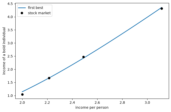
Fig. 55.5 The bold type’s sharing rule#
The first-best sharing rule is convex, while shares in firms of almost the same size give the bold type an income that is close to affine in income per person.
The four points lie close to the curve, which is why the loss from the stock market is so small.
55.8.3. When is the equilibrium first-best?#
Proposition 8 of Kihlstrom and Laffont [1982] gives two cases in which a stock market equilibrium is first-best efficient: when all individuals are alike, and when risk-neutral individuals are numerous and wealthy enough to hold all of the economy’s firms, which Exercise 55.3 asks you to study.
Exercise 55.2 gives two more, constant absolute risk aversion and quadratic utility.
Another case arises when there are only two states.
econ_two = create_economy(z=(0.5, 2.0), θ=(0.2, 0.8), p=(0.5, 0.5))
r_two, sol_two = solve_stock_market(econ_two)
print(f"two states: price of capital {r_two:.4f}")
for i, (K, C) in enumerate(sol_two):
    marg_u = econ_two.utilities[i].du(incomes(K, C, r_two, econ_two))
    print(f"{names[i]:9s}: K = {K:.5f}, C = {C:.3f}, "
          f"marginal rate of substitution {marg_u[1] / marg_u[0]:.5f}")
two states: price of capital 0.5498
bold     : K = 2.02080, C = 2.933, marginal rate of substitution 0.58663
cautious : K = 2.02080, C = 0.356, marginal rate of substitution 0.58663
With the low- and high-productivity states of our example as the only states, each with probability \(1/2\), both types choose the same operating capital, and their marginal rates of substitution are equal.
This two-state economy has no state with zero output, so the bankruptcy constraint that we impose is stricter than nonnegative income requires, but it does not bind.
With two states, a safe claim and equity in firms that operate at a common \(K\) span all state-contingent payoffs, so markets are effectively complete.
Moreover, every investor wants firms to operate at the same \(K\), whatever its preferences.
When its bankruptcy constraint does not bind, an investor’s income is \(A + r + C \, d(K, x)\), where \(d(K, x) = y(K, x) - r\) is the excess return on equity capital, which in equilibrium is negative in the low-productivity state \(x_1\) and positive in the high-productivity state \(x_2\).
So an investor who supplies equity capital wants the \(K\) that gives the most income in state \(x_2\) per unit of income given up in state \(x_1\), the \(K\) that maximizes \(d(K, x_2) / [-d(K, x_1)]\), because any other \(K\) is dominated.
Given \(r\), every type therefore chooses the same \(K\), and its first-order condition for \(C\), \(\sum_x p(x) u_i'(c_i(x)) \, d(K, x) = 0\), gives every type the same ratio of state prices, \(-d(K, x_1) / d(K, x_2)\).
Equivalently, with two states every discount factor is an affine function of \(y\), so the mean-variance argument above holds exactly.
All firms then operate at the same \(K\), marginal rates of substitution are equal, and the equation for the price of capital (55.7) is the third condition for first-best efficiency, so the equilibrium is first-best efficient.
With more than two states, as in our main example, the two assets no longer span the states, and the equilibrium is generally not first-best efficient.
55.9. The value of a stock market#
The economy without a stock market is not efficient even in Diamond’s restricted sense, so a planner with access to a stock market could make everybody better off.
To see how much a stock market accomplishes, we compare three market structures:
no stock market, as in Kihlstrom and Laffont [1979],
a stock market, as in Kihlstrom and Laffont [1982], and
complete markets, in which individuals can also trade a claim to one unit of income in each state, an Arrow security.
With complete markets, the equilibrium is the first-best allocation at which each type can just afford its incomes with the value of its endowment.
Let \(Q(x)\) be the price of an Arrow security that pays in state \(x\), normalized so that a sure unit of income costs \(1\).
A firm that operates at \(K\) is worth \(\sum_x Q(x) g(K, x)\), so free entry makes the price of capital \(r = \max_K \sum_x Q(x) g(K, x) / (1 + K)\), and each type’s budget constraint is \(\sum_x Q(x) c_i(x) = A + r\).
In a first-best allocation, \(Q(x)\) is proportional to \(p(x) u_i'(c_i(x))\), the same for both types, and we search for the weight \(w\) at which the bold type’s budget constraint holds.
Because \(K^0\) maximizes the weighted sum of expected utilities, it satisfies \(\sum_x Q(x) \, y_K(K^0, x) = 0\), so it satisfies the first-order condition for maximizing the value of output per unit of capital at the prices \(Q\), and in our example it is the maximizer, so \(r = \sum_x Q(x) \, y(K^0, x)\).
This computation follows the strategy of Cass-Koopmans Competitive Equilibrium, which applies the “big \(K\), little \(k\)” device to a planning problem.
We solve a planning problem, the first-best problem with weight \(w\) on the bold type, and treat its allocation as big \(K\).
We read the prices \(Q\) off the planner’s marginal utilities and the price \(r\) off the free-entry condition.
At these prices every type’s planned incomes satisfy its first-order conditions, but, unlike the representative household of Cass-Koopmans Competitive Equilibrium, a type can afford them only for the right weight \(w\), which we find by the method of Negishi [1960].
def complete_markets(econ):
    "Equilibrium with a complete set of Arrow securities."
    u_2 = econ.utilities[1]
    # big K: the first-best allocation with weight w, and its prices
    def allocation_and_prices(w):
        K_0, c_1, c_2 = efficient_allocation(w, econ)
        Q = econ.p * u_2.du(c_2)
        Q = Q / Q.sum()
        r = Q @ output_per_capital(K_0, econ)
        return K_0, c_1, c_2, r, Q
    # Negishi: find the w at which type 1 can just afford its planned
    # incomes; type 2's budget constraint then holds by Walras's law
    def budget_gap(w):
        _, c_1, _, r, Q = allocation_and_prices(w)
        return Q @ c_1 - (econ.A + r)
    w = brentq(budget_gap, 1e-3, 1 - 1e-3, xtol=1e-12)
    return allocation_and_prices(w)

K_cm, c_1_cm, c_2_cm, r_cm, _ = complete_markets(econ)

def summary(r, firms, K, v, econ):
    "Table column: price, firms, firm sizes, output, certainty equivalents."
    output = sum(n * (econ.p @ g(K_i, econ)) for n, K_i in zip(firms, K))
    ce = [certainty_equivalent(v_i, ut) for v_i, ut in zip(v, econ.utilities)]
    return [r, sum(firms), *K, output, *ce]

K_ns = [entrepreneur_K(r_ns, ut, econ) for ut in econ.utilities]
K_sm = [K for K, C in solutions]
ν_sm = [C / (1 + K) * μ_i for (K, C), μ_i in zip(solutions, econ.μ)]
v_cm = [econ.p @ ut.u(c) for ut, c in zip(econ.utilities, (c_1_cm, c_2_cm))]
table = pd.DataFrame({
    'no stock market': summary(r_ns, entrepreneurs_ns, K_ns, v_ns, econ),
    'stock market': summary(r_sm, ν_sm, K_sm, v_sm, econ),
    # all firms are alike, so assign them all to the first entry
    'complete markets': summary(r_cm, [1 / (1 + K_cm), 0], [K_cm, K_cm],
                                v_cm, econ)},
    index=['price of capital', 'number of firms',
           'operating capital, bold firms',
           'operating capital, cautious firms',
           'expected output per person',
           'certainty-equivalent income, bold',
           'certainty-equivalent income, cautious'])
table.round(4)
| no stock market | stock market | complete markets | |
|---|---|---|---|
| price of capital | 0.4260 | 0.4948 | 0.4957 |
| number of firms | 0.3606 | 0.3910 | 0.3908 |
| operating capital, bold firms | 2.2828 | 1.5661 | 1.5588 |
| operating capital, cautious firms | 0.6207 | 1.5348 | 1.5588 |
| expected output per person | 0.5641 | 0.5752 | 0.5752 |
| certainty-equivalent income, bold | 2.7515 | 2.6119 | 2.6104 |
| certainty-equivalent income, cautious | 2.4260 | 2.5087 | 2.5094 |
With complete markets all firms are alike, so the two rows for operating capital coincide in the last column.
Without a stock market, firms are too dispersed in size and too few, and expected output is about 2 percent lower than with complete markets.
The stock market closes almost all of the gap: its price of capital, number of firms, firm sizes, expected output, and certainty equivalents are all close to their complete-markets values.
The bold type is even slightly better off with a stock market than with complete markets, and the cautious type slightly worse off, because the two market structures divide the gains from trade differently.
The stock market also redistributes.
In this example it raises the price of capital.
The cautious type, a net seller of capital, gains: without a stock market it is the marginal type, so its welfare is \(u_2(A + r)\) at the lower price, while with a stock market it could sell its capital at the higher price, and it does better still by holding some equity.
The bold type, a net buyer of capital, loses, because the higher price that it pays for capital outweighs its gain from sharing risk.
55.9.1. Who gains?#
Who gains from a stock market depends on the composition of the population.
Fig. 55.6 varies the share of bold individuals, keeping everything else the same, and shows the price of capital with and without a stock market, and each type’s gain in certainty-equivalent income from opening a stock market.
bold_shares = np.linspace(0.05, 0.95, 37)
results = []
for μ_bold in bold_shares:
    e = create_economy(μ=(μ_bold, 1 - μ_bold))
    r_n, _, _ = solve_no_stock_market(e)
    r_s, sol = solve_stock_market(e)
    gains = []
    for ut, (K, C) in zip(e.utilities, sol):
        with_market = e.p @ ut.u(incomes(K, C, r_s, e))
        without = max(entrepreneur_value(r_n, ut, e), ut.u(e.A + r_n))
        gains.append(certainty_equivalent(with_market, ut)
                     - certainty_equivalent(without, ut))
    results.append([r_n, r_s, *gains])
results = np.array(results)

fig, axes = plt.subplots(1, 2, figsize=(11, 4.5))
axes[0].plot(bold_shares, results[:, 0], lw=2, label='no stock market')
axes[0].plot(bold_shares, results[:, 1], lw=2, label='stock market')
for r_i in r_ce:
    axes[0].axhline(r_i, color='gray', ls=':', lw=1)
axes[0].set_ylabel('price of capital $r$')
axes[1].plot(bold_shares, results[:, 2], lw=2, label='bold')
axes[1].plot(bold_shares, results[:, 3], lw=2, label='cautious')
axes[1].axhline(0, color='k', lw=1)
axes[1].set_ylabel('gain in certainty-equivalent income')
for ax in axes:
    ax.axvline(econ.μ[0], color='k', ls='--', lw=1)
    ax.set_xlabel(r'share of bold individuals $\mu_1$')
    ax.legend()
plt.tight_layout()
plt.show()
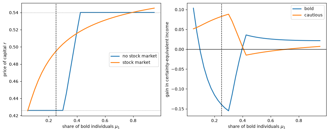
Fig. 55.6 Effects of opening a stock market#
The dotted lines in the left panel mark the two types’ certainty-equivalent prices, and the dashed lines mark the share of bold individuals in our example.
Without a stock market, the price of capital has three regions.
When bold individuals make up less than about 30 percent of the population, the cautious type is marginal, and the price equals the cautious type’s certainty-equivalent price.
When they make up more than about 42 percent, the bold type is marginal, and the price equals the bold type’s certainty-equivalent price.
In between, all bold individuals and no cautious ones are entrepreneurs, and the price rises with the share of bold individuals.
In both economies, every individual can sell its capital at the price \(r\), so its welfare is at least \(u_i(A + r)\), and a type that is marginal or a capitalist without a stock market gets exactly \(u_i(A + r)\).
So when the stock market raises the price of capital, the types that are marginal or capitalists without it gain, and when it lowers the price of capital, they can lose.
The stock market raises the price of capital when bold individuals make up between about 5 and 40 percent of the population, lowers it when they make up between about 40 and 80 percent, and raises it again above about 80 percent.
When their share is between about 10 and 40 percent, the bold, who are entrepreneurs without a stock market, lose.
When it is between about 40 and 70 percent, the cautious, who are then all capitalists without a stock market, lose.
Both types gain at other shares, including a narrow band around 40 percent: where the stock market leaves the price of capital nearly unchanged, everybody gains from sharing risk.
55.10. Two special cases#
55.10.1. Stochastic constant returns to scale#
Suppose that \(g(K, x) = h(K) \, x\) with \(x\) a scalar, which is what Diamond [1967] called stochastic constant returns to scale.
Then output per unit of capital is \(x \, h(K) / (1 + K)\), and every investor, whatever its attitude toward risk, maximizes \(h(K) / (1 + K)\), so that every firm operates at \(K^\ast\).
This is the unanimity result of Leland [1974] and Ekern and Wilson [1974]: every shareholder of every firm wants the firm to maximize its market value.
In this case, the equilibrium is Diamond’s, capital is allocated across firms as in a first-best allocation, and the number of firms, \(1 / (1 + K^\ast)\), is the first-best number; only the allocation of risk remains inefficient.
The next cell checks that both types choose \(K^\ast = 1\) when \(\theta = 0.5\) in every state, so that \(h(K) = K^{0.5}\) and \(x = z\).
econ_scrs = create_economy(θ=(0.5, 0.5, 0.5, 0.5))
r_scrs, sol_scrs = solve_stock_market(econ_scrs)
print(f"K* = {K_star(econ_scrs):.4f}, operating capital by type: "
      f"{sol_scrs[0][0]:.4f} and {sol_scrs[1][0]:.4f}, "
      f"price of capital {r_scrs:.4f}")
K* = 1.0000, operating capital by type: 1.0000 and 1.0000, price of capital 0.4937
Kihlstrom and Laffont also point out that free entry makes the economy’s technology a cone, because a firm can be replicated without limit at the cost of one unit of capital, so their technology has stochastic constant returns to scale in a broader sense.
55.10.2. No uncertainty#
Without uncertainty, the investor’s problem (55.6) is solved by the \(K\) that maximizes output per unit of capital, which minimizes average cost.
Competition then drives the price of capital to the maximized output per unit of capital, which equals the marginal product of capital at \(K^\ast\) by (55.2).
The equilibrium is the long-run competitive equilibrium in which free entry drives profits to zero and firms produce at minimum average cost.
55.11. When is a stock market needed?#
Section 5.8 of Kihlstrom and Laffont [1982] argues that a stock market is needed only when three conditions hold.
Set-up costs: if creating a firm were free, every investor could create a firm of the size it wants and hold all of it, so no shares would need to be traded.
Uncertainty: without uncertainty, entrepreneurs can buy all of their operating capital and capitalists can sell it, and every individual receives \(A + r\) with or without a stock market.
Risk aversion: if there are enough risk-neutral individuals, and if each of them can set up more than one firm, they can hold all firms, and the risk averse can simply sell their capital.
Stiglitz [1974] and Newbery [1977] had made the first point in models of sharecropping without fixed costs, in which a market for shares of output is unnecessary.
The same three features, fixed costs, risk, and risk aversion, are what make the choice between being an entrepreneur and being a capitalist interesting in Kihlstrom and Laffont [1979].
55.13. Connections to other lectures#
Irrelevance of Capital Structures with Complete Markets and Equilibrium Capital Structures with Incomplete Markets study a two-period economy in which a representative firm chooses its capital and its debt.
With complete markets, the Modigliani-Miller theorem makes the firm’s financial structure indeterminate in those lectures, while with incomplete markets and defaultable debt, the aggregate financial structure is determinate.
Kihlstrom and Laffont obtain the Modigliani-Miller theorem from free entry with incomplete markets, and because their bankruptcy constraint makes debt riskless, both individual and aggregate financial structures are indeterminate.
In Equilibrium Capital Structures with Incomplete Markets, a capital and debt choice that no firm makes is priced at the highest valuation that any type of investor places on it, and the firm chooses its capital and debt to maximize its market value at those prices.
In Kihlstrom and Laffont’s model, free entry instead caps the price of any firm at its replication cost \(1 + K - B\), and clienteles replace a firm objective, because each firm is run as its own shareholders want it run.
Their price expectations \(N(K, B)\) for firms that nobody creates play the role of the rational conjectures of Bisin et al. [2018] and Makowski [1983].
Rational Expectations Equilibrium introduces the “big \(K\), little \(k\)” device that we use to compute the equilibria in this lecture, and Investment Under Uncertainty and Cass-Koopmans Competitive Equilibrium apply it; in those lectures firms or households are identical, so consistency means that little \(k\) equals big \(K\), while here individuals of different types choose differently, and consistency means that their choices clear markets.
Corporate Financial Structure and Managerial Incentives studies a firm whose manager, not its owners, chooses investment and financial structure, so that the Modigliani-Miller theorem fails.
Competitive Equilibria with Arrow Securities computes competitive equilibria with complete markets in Arrow securities, like the complete-markets benchmark in our comparison of market structures.
Elementary Asset Pricing Theory describes asset pricing with a stochastic discount factor; in (55.7), each type’s discount factor values capital’s marginal product and output per unit of capital.
Gorman Aggregation studies Gorman aggregation, in which each household’s consumption is a household-specific linear function of aggregate consumption; with the preferences of Exercise 55.2, shares in identical firms deliver sharing rules of this kind, which is why the stock market equilibrium is then first-best.
Coase’s Theory of the Firm presents a theory in which transaction costs determine the boundary of a firm; here a firm’s size is determined instead by the fixed cost of creating it, diminishing returns, and the attitudes toward risk of the investors who own it.
55.14. Exercises#
Exercise 55.1
Theorem 4 of Kihlstrom and Laffont [1979] shows that, when all entrepreneurs are identical and technology satisfies some further conditions, an increase in everybody’s risk aversion lowers the equilibrium wage, their counterpart of our price of capital, because, at a given wage, more individuals choose the safe role and entrepreneurs run smaller firms.
Multiply both types’ relative risk aversion by a factor \(\lambda\), so that the types have relative risk aversion \(0.5 \lambda\) and \(4 \lambda\), keeping everything else as in the lecture.
For \(\lambda\) between \(0.5\) and \(2\), compute the price of capital and the number of firms with and without a stock market, and plot them against \(\lambda\).
Explain the results.
Solution
λ_grid = np.linspace(0.5, 2.0, 13)
rows = []
for λ in λ_grid:
    e = create_economy(ρ=(0.5 * λ, 4.0 * λ))
    r_n, ents, _ = solve_no_stock_market(e)
    r_s, sol = solve_stock_market(e)
    firms_s = sum(C / (1 + K) * μ_i for (K, C), μ_i in zip(sol, e.μ))
    rows.append([r_n, r_s, ents.sum(), firms_s])
rows = np.array(rows)

fig, axes = plt.subplots(1, 2, figsize=(11, 4.5))
for j, label in enumerate(['no stock market', 'stock market']):
    axes[0].plot(λ_grid, rows[:, j], lw=2, label=label)
    axes[1].plot(λ_grid, rows[:, 2 + j], lw=2, label=label)
axes[0].set_ylabel('price of capital $r$')
axes[1].set_ylabel('number of firms')
for ax in axes:
    ax.set_xlabel(r'scale of risk aversion $\lambda$')
    ax.legend()
plt.tight_layout()
plt.show()
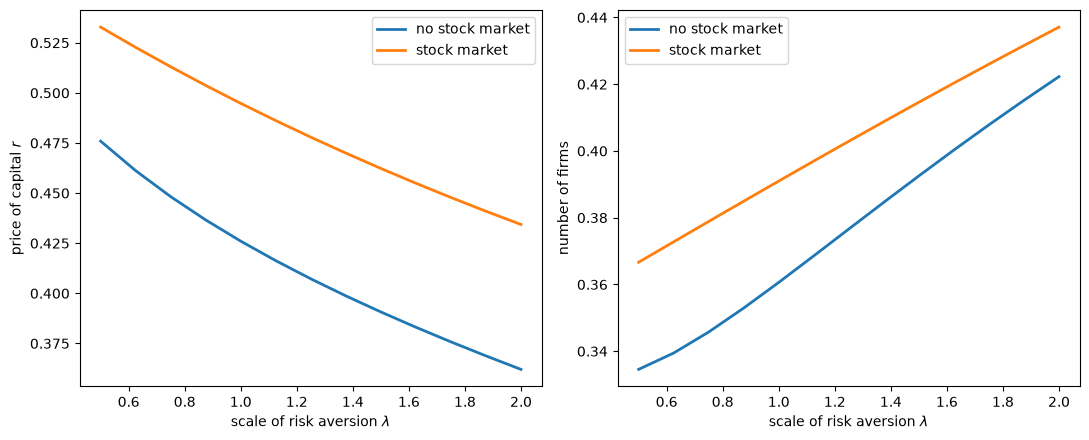
In both economies, more risk aversion lowers the price of capital and raises the number of firms.
Without a stock market, the conclusion is immediate in our example: at every \(\lambda\) on the grid, all bold individuals are entrepreneurs and the cautious type is marginal, so the price of capital equals the cautious type’s certainty-equivalent price, which falls as its risk aversion rises.
Theorem 4 of Kihlstrom and Laffont [1979] does not apply directly, because bold and cautious entrepreneurs coexist, but the same two forces are at work: at a given price, fewer individuals want to be entrepreneurs, and entrepreneurs run smaller firms.
With a stock market, more risk aversion lowers every type’s demand for equity capital at any price, so the price of capital must fall to clear the market, and investors want the firms they own to operate at smaller scales.
In both economies, the supply of capital is fixed at one unit, so smaller firms mean more of them: the number of firms is one divided by one plus the average operating capital per firm.
So, although fewer individuals want to be entrepreneurs at a given price, the number of entrepreneurs without a stock market rises in equilibrium, because the price of capital falls and each entrepreneur runs a smaller firm.
As in the lecture, the stock market raises the price of capital at every \(\lambda\) on the grid.
Exercise 55.2
This exercise studies two classes of preferences for which every type chooses the same operating capital, keeping the four-state technology of the lecture.
Suppose that both types have constant absolute risk aversion, \(u_i(c) = -\exp(-a_i c)\), with \(a_1 = 0.5\) and \(a_2 = 3\); compute the equilibrium, and show that both types choose the same operating capital \(\bar K\), which differs from \(K^\ast\).
Show that the shares \(\gamma_i\) are proportional to the types’ risk tolerances \(1/a_i\).
Note 2 of Kihlstrom and Laffont [1982] shows that \(\bar K\) solves
\[ E \left\{ \left[ g_K(\bar K, \tilde x) - \frac{g(\bar K, \tilde x)}{1 + \bar K} \right] \exp \left[ - \bar a \, \frac{g(\bar K, \tilde x)}{1 + \bar K} \right] \right\} = 0, \qquad \bar a = \left( \sum_i \frac{\mu_i}{a_i} \right)^{-1} \]Verify this numerically.
Is the equilibrium first-best efficient?
Now suppose instead that both types have quadratic utility, \(u_i(c) = -(\beta_i - c)^2 / 2\), with bliss points \(\beta_1 = 12\) and \(\beta_2 = 4\), which are above every income that the types receive in equilibrium; show that both types choose the same operating capital and have the same marginal rates of substitution, and explain why, using the mean-variance argument of the lecture.
Solution
def cara(a):
    "Constant absolute risk aversion a."
    return Utility(u=lambda c: -np.exp(-a * c),
                   du=lambda c: a * np.exp(-a * c))

a = np.array([0.5, 3.0])
econ_cara = econ._replace(utilities=[cara(a_i) for a_i in a])
r_cara, sol_cara = solve_stock_market(econ_cara)
print(f"price of capital {r_cara:.4f}, K* = {K_s:.4f}")
for i, (K, C) in enumerate(sol_cara):
    marg_u = econ_cara.utilities[i].du(incomes(K, C, r_cara, econ_cara))
    print(f"type {i + 1}: K = {K:.5f}, γ = {C / (1 + K):.4f}, "
          f"γ times a_i = {a[i] * C / (1 + K):.4f}, "
          f"marginal rates of substitution {np.round(marg_u / marg_u[0], 5)}")

a_bar = 1 / (econ_cara.μ @ (1 / a))
def note_2_condition(K, a_bar, econ):
    "Left side of the equation for the common K in Note 2."
    y = output_per_capital(K, econ)
    return econ.p @ ((g_K(K, econ) - y) * np.exp(-a_bar * y))

K_bar = brentq(note_2_condition, 0.1, K_s, args=(a_bar, econ_cara))
print(f"K from note 2: {K_bar:.5f}")
price of capital 0.4182, K* = 1.9224
type 1: K = 1.16210, γ = 1.2334, γ times a_i = 0.6167, marginal rates of substitution [1.      0.72779 0.51438 0.24886]
type 2: K = 1.16210, γ = 0.2056, γ times a_i = 0.6167, marginal rates of substitution [1.      0.72779 0.51438 0.24886]
K from note 2: 1.16210
Both types choose the same operating capital, which is smaller than \(K^\ast\), and \(\gamma_i a_i\) is the same for both types, so the shares are proportional to risk tolerance.
The reason is that, when the bankruptcy constraint does not bind, as here, a type’s problem (55.6) depends on \(a_i\) and \(C\) only through their product: income is \(A + r + C \, [g(K, \tilde x)/(1 + K) - r]\), and \(-\exp(-a_i \cdot \text{income})\) depends on \(C\) only through \(a_i C\).
So every type chooses the same \(K\) and the same \(a_i C_i\), the portfolio separation that Section 5.9 of Kihlstrom and Laffont [1982] mentions, and market clearing, \(\sum_i \mu_i C_i = 1\), gives \(a_i C_i = \bar a\).
The equilibrium is first-best efficient, even though there are four states.
Each type’s income in state \(x\) is a constant plus \((\bar a / a_i) \, g(\bar K, x) / (1 + \bar K)\), so its marginal rate of substitution between states \(x\) and \(x'\) is \(\exp\{-\bar a \, [g(\bar K, x) - g(\bar K, x')] / (1 + \bar K)\}\), the same for every type, as the printed values confirm.
All firms operate at \(\bar K\), and the first-order condition for \(K\) is the third condition for first-best efficiency.
With constant absolute risk aversion, efficient risk sharing requires only that each individual receive a fraction of the economy’s risky output proportional to its risk tolerance \(1/a_i\), which shares in identical firms provide.
Now quadratic utility.
def quadratic(β):
    "Quadratic utility with bliss point β."
    return Utility(u=lambda c: -(β - c)**2 / 2, du=lambda c: β - c)

econ_quad = econ._replace(utilities=[quadratic(12.0), quadratic(4.0)])
r_quad, sol_quad = solve_stock_market(econ_quad)
print(f"price of capital {r_quad:.4f}")
for i, (K, C) in enumerate(sol_quad):
    c = incomes(K, C, r_quad, econ_quad)
    marg_u = econ_quad.utilities[i].du(c)
    print(f"type {i + 1}: K = {K:.6f}, C = {C:.3f}, "
          f"highest income {c.max():.3f}, "
          f"marginal rates of substitution {np.round(marg_u / marg_u[0], 5)}")
price of capital 0.5298
type 1: K = 1.696104, C = 2.729, highest income 4.173, marginal rates of substitution [1.      0.94847 0.87924 0.71699]
type 2: K = 1.696104, C = 0.424, highest income 2.785, marginal rates of substitution [1.      0.94847 0.87924 0.71699]
Both types choose the same operating capital, and their marginal rates of substitution are equal.
With quadratic utility, marginal utility \(\beta_i - c\) is linear in income, so the stochastic discount factor is exactly \(m_i(x) = 1 - b_i [y(K_i, x) - E y(K_i, \tilde x)]\), with \(b_i = C_i / (\beta_i - E c_i)\).
The mean-variance argument of the lecture is then exact: the first-order conditions give \(b_i = (E y - r) / \operatorname{Var}(y)\) and a preference-free equation for \(K\), which has a single relevant root here, so every type chooses the same \(K\) and has the same \(b_i\), and hence the same discount factor.
As with constant absolute risk aversion, all firms operate at the same scale, marginal rates of substitution are equal, and (55.7) is the third condition for first-best efficiency, so the equilibrium is first-best efficient.
Exercise 55.3
Replace the bold type with risk-neutral individuals, \(u_1(c) = c\), and let their measure \(\mu_1\) vary, keeping the cautious type and the technology of the lecture.
According to Proposition 6 and Theorem 1 of Kihlstrom and Laffont [1982], if
then \(r = E g(K^\ast, \tilde x) / (1 + K^\ast)\), all firms operate at \(K^\ast\), risk-neutral individuals hold all of them, and the risk averse hold none.
Compute the threshold for \(\mu_1\).
Compute the equilibrium price of capital for a grid of values of \(\mu_1\) between \(0.02\) and \(0.5\), and plot it.
Explain why the equilibrium is first-best efficient above the threshold.
Solution
A risk-neutral investor supplies as much equity capital as the bankruptcy constraint allows, \(C_1 = A/r + 1\), when \(r\) is below \(E g(K^\ast, \tilde x)/(1 + K^\ast)\), the maximal expected output per unit of capital, and is indifferent when \(r\) equals it.
So we solve for the equilibrium directly: if risk-neutral investors can absorb all of the capital at \(r = E g(K^\ast, \tilde x)/(1 + K^\ast)\), that is the equilibrium price; otherwise the price is the one at which the market for equity capital clears with the risk-neutral investors at their bound.
threshold = 1 / (econ.A / (econ.p @ g_K(K_s, econ)) + 1)
print(f"threshold for μ_1: {threshold:.4f}")

def equilibrium_with_risk_neutral(μ_1, econ):
    "Price of capital when risk-neutral types of measure μ_1 join the cautious."
    r_top = econ.p @ output_per_capital(K_star(econ), econ)
    cautious = econ.utilities[1]
    def excess(r):
        C_2 = solve_investor(r, cautious, econ)[1]
        return μ_1 * (econ.A / r + 1) + (1 - μ_1) * C_2 - 1
    r_hi = (1 - 1e-9) * r_top
    # can the risk-neutral investors hold every firm at r_top?  By esm-kstar,
    # this is the same as μ_1 >= threshold, but testing excess demand directly
    # is robust to rounding error in the numerically computed K*
    if excess(r_hi) >= 0:
        return r_top
    return brentq(excess, 0.05 * r_top, r_hi, xtol=1e-12)

μ_grid = np.sort(np.append(np.linspace(0.02, 0.5, 25), threshold))
r_values = [equilibrium_with_risk_neutral(μ_1, econ) for μ_1 in μ_grid]

fig, ax = plt.subplots(figsize=(8, 5))
ax.plot(μ_grid, r_values, lw=2)
ax.axhline(r_max, color='gray', ls=':', lw=1.5,
           label=r'$E\,g(K^*, x) / (1 + K^*)$')
ax.axvline(threshold, color='k', ls='--', lw=1, label='threshold')
ax.set_xlabel(r'measure of risk-neutral individuals $\mu_1$')
ax.set_ylabel('price of capital $r$')
ax.legend()
plt.show()
threshold for μ_1: 0.2241
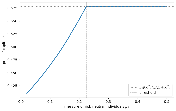
Below the threshold, risk-neutral investors cannot hold all of the firms without risking negative income in the state in which output is zero, so risk-averse investors must be induced to hold some shares, and the price of capital falls below expected output per unit of capital.
Above the threshold, risk-neutral investors hold every firm, all firms operate at the risk-neutral scale \(K^\ast\), and the risk averse receive the safe income \(A + r\).
All risk is then borne by individuals who are indifferent to it, which is an efficient allocation of risk, all firms operate at the same scale, and with risk-neutral owners the condition for the number of firms reduces to (55.2), so all three conditions for first-best efficiency hold, as Proposition 8 of Kihlstrom and Laffont [1982] states.
Exercise 55.4
Section 5.7 of Kihlstrom and Laffont [1982] conjectures that, with nonclassical price expectations, there is a profusion of equilibria.
Pick a level \(\hat K\) of operating capital, and suppose that \(N(K, B) = N_c(K, B)\) when \(K = \hat K\) and \(N(K, B) = 0\) otherwise, so that nobody expects to sell shares in a firm that operates at any other level.
In a candidate equilibrium, every firm operates at \(\hat K\), each type chooses only how much equity capital \(C\) to supply, and \(r\) clears the market for equity capital.
The candidate is an equilibrium if no individual gains by creating a firm at some other \(K\), holding all of it, and supplying equity capital to the firms at \(\hat K\).
For \(\hat K\) between \(0.3\) and \(2\), compute the candidate equilibrium and each type’s largest gain in certainty-equivalent income from such a deviation.
Which values of \(\hat K\) can be equilibria? Explain why the answer depends on the bold type’s \(\gamma > 1\).
Repeat the computation for an economy in which everybody is of the cautious type, and compare the equilibria that you find with the equilibrium with classical expectations.
Solution
def single_K_equilibrium(K_hat, econ):
    "Price of capital and each type's equity capital if every firm uses K_hat."
    y = output_per_capital(K_hat, econ)

    def equity(r, ut):
        def f(C):
            return -(econ.p @ ut.u(econ.A + r * (1 - C) + C * y))
        return minimize_scalar(f, bounds=(0, econ.A / r + 1),
                               method='bounded', options={'xatol': 1e-12}).x

    def excess(r):
        return econ.μ @ [equity(r, ut) for ut in econ.utilities] - 1

    r_top = econ.p @ y
    r = brentq(excess, 0.05 * r_top, (1 - 1e-9) * r_top, xtol=1e-13)
    return r, [equity(r, ut) for ut in econ.utilities]

def deviation_gain(K_hat, r, C, ut, econ):
    """
    Gain in certainty-equivalent income from creating a firm at some K,
    holding all of it, and supplying equity capital C_d to firms at K_hat.
    """
    y_hat = output_per_capital(K_hat, econ)

    def value(K, C_d):
        income = econ.A - r * (K + C_d) + g(K, econ) + C_d * y_hat
        return econ.p @ ut.u(income)

    def best_C_d(K):
        # income must stay positive in the state in which output is zero
        return minimize_scalar(lambda C_d: -value(K, C_d),
                               bounds=(0, econ.A / r - K - 1e-9),
                               method='bounded',
                               options={'xatol': 1e-12}).x

    K_d = minimize_scalar(lambda K: -value(K, best_C_d(K)),
                          bounds=(1e-6, econ.A / r - 1e-6), method='bounded',
                          options={'xatol': 1e-12}).x
    v_deviate = value(K_d, best_C_d(K_d))
    v_stay = econ.p @ ut.u(econ.A + r * (1 - C) + C * y_hat)
    return (certainty_equivalent(v_deviate, ut)
            - certainty_equivalent(v_stay, ut))

def max_gains(K_hat, econ):
    "Each type's largest gain from deviating when every firm uses K_hat."
    r, equities = single_K_equilibrium(K_hat, econ)
    return [deviation_gain(K_hat, r, C, ut, econ)
            for C, ut in zip(equities, econ.utilities)]

econ_cautious = create_economy(ρ=(4.0,), μ=(1.0,))
K_hat_grid = np.linspace(0.3, 2.0, 18)
gains = np.array([max_gains(K_hat, econ) for K_hat in K_hat_grid])
gains_cautious = [max_gains(K_hat, econ_cautious)[0] for K_hat in K_hat_grid]

fig, axes = plt.subplots(1, 2, figsize=(11, 4.5))
for i, name in enumerate(names):
    axes[0].plot(K_hat_grid, gains[:, i], lw=2, label=name)
axes[0].set_title('two types')
axes[1].plot(K_hat_grid, gains_cautious, lw=2, label='cautious')
axes[1].set_title('everybody cautious')
for ax in axes:
    ax.axhline(0, color='k', lw=1)
    ax.set_xlabel(r'operating capital of every firm $\hat K$')
    ax.set_ylabel('largest gain from deviating')
    ax.legend()
plt.tight_layout()
plt.show()

K_nc = minimize_scalar(lambda K_hat: max_gains(K_hat, econ)[0],
                       bounds=(1.4, 1.7), method='bounded',
                       options={'xatol': 1e-8}).x
r_nc, equities_nc = single_K_equilibrium(K_nc, econ)
print(f"two types: K_hat = {K_nc:.4f}, bold equity capital "
      f"{equities_nc[0]:.3f} > 1 + K_hat")
print(f"bold firms with classical expectations: K = {solutions[0][0]:.4f}")
for i, ut in enumerate(econ.utilities):
    v_nc = econ.p @ ut.u(incomes(K_nc, equities_nc[i], r_nc, econ))
    print(f"  {names[i]:9s}: certainty-equivalent income "
          f"{certainty_equivalent(v_nc, ut):.5f}, "
          f"classical {certainty_equivalent(v_sm[i], ut):.5f}")
r_c, ((K_c, _),) = solve_stock_market(econ_cautious)
print(f"everybody cautious: classical K = {K_c:.4f}")
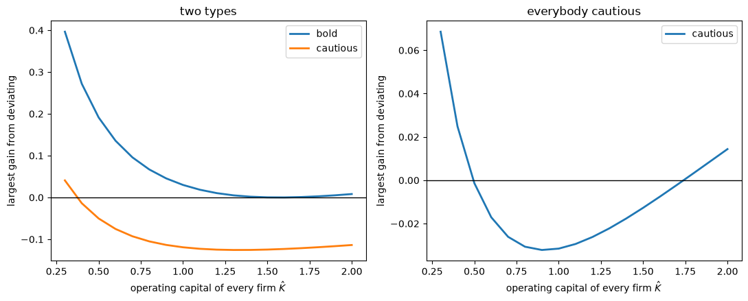
two types: K_hat = 1.5656, bold equity capital 2.937 > 1 + K_hat
bold firms with classical expectations: K = 1.5661
  bold     : certainty-equivalent income 2.61214, classical 2.61190
  cautious : certainty-equivalent income 2.50857, classical 2.50866
everybody cautious: classical K = 1.0956
The cautious type gains from deviating only when \(\hat K\) is below about \(0.4\): otherwise a whole firm, which requires about \(2.5\) units of equity capital, is far more risk than it wants to bear, since it supplies only about \(0.35\) units.
The bold type supplies about \(2.94\) units of equity capital, more than the \(1 + \hat K\) units that a whole firm requires.
So it can create a firm at a \(K\) close to \(\hat K\), hold all of it, and keep the rest of its equity capital in firms at \(\hat K\), a small change in its portfolio.
The bold type therefore gains unless \(\hat K\) satisfies its own first-order condition for \(K\), and only \(\hat K \approx 1.566\) survives, almost exactly the operating capital of bold firms with classical expectations.
In that equilibrium, nobody creates firms run as the cautious type would run them, because nobody expects to be able to sell their shares, an expectation that is never tested.
The bold type gains slightly and the cautious type loses slightly relative to the equilibrium with classical expectations.
When everybody is cautious, each individual supplies one unit of equity capital, less than the \(1 + \hat K\) units of a whole firm, so every deviation is a large and risky change in its portfolio.
Every \(\hat K\) between about \(0.49\) and \(1.74\) then survives, the profusion of equilibria that Kihlstrom and Laffont conjecture.
With one type, everybody’s income in such an equilibrium is \(A + g(\hat K, \tilde x)/(1 + \hat K)\), whose expected utility is highest at the operating capital \(K = 1.096\) chosen with classical expectations, so every other equilibrium makes everybody worse off, as Kihlstrom and Laffont conjecture.