56. Corporate Financial Structure and Managerial Incentives#
56.1. Overview#
The Modigliani-Miller theorem [Modigliani and Miller, 1958] says that the market value of a firm does not depend on how the firm divides its financing between debt and equity.
The theorem rests on an assumption that is easy to overlook: the firm’s production plan does not depend on its financial structure.
Grossman and Hart [1982] study a widely held corporation in which that assumption fails.
The corporation is run by a manager whose goals, such as enjoying perquisites, conflict with the shareholders’ goal of a high market value.
Investors cannot observe how much of the money they provide the manager invests and how much the manager spends on perquisites.
What disciplines the manager is the threat of bankruptcy, which costs the manager the perquisites of the job.
Grossman and Hart begin with a thought experiment.
Suppose that a project costs $100 and returns a stream of profits worth $100, so that its net present value is zero, as free entry requires.
If the firm raises the $100 by issuing equity, nothing prevents its manager from canceling the project and spending the money on perquisites; the shareholders simply lose their $100.
If the firm raises the $100 by issuing debt, any choice other than the profit-maximizing plan leads to bankruptcy for sure.
So whether competition forces a firm to maximize profits depends on its financial structure.
In a mature corporation, though, it is management, not the shareholders, that controls the financial structure, and since debt raises the probability of bankruptcy, it might seem that management would never issue debt.
Grossman and Hart’s answer is that debt lets management precommit, or bond itself, to pursue profits.
Because investors know that a heavily indebted manager has a strong incentive to avoid bankruptcy, they value the firm more highly, so a manager who wants a high market value issues debt.
Managers can want a high market value for at least three reasons.
Their salaries may depend on it.
A higher market value makes a takeover bid less likely, because a raider must pay more for the firm.
A higher market value lets them raise more capital, and more capital means more perquisites.
The main model of Grossman and Hart [1982] focuses on the third reason, and an extension takes up the second, drawing on their earlier analysis of takeover bids in Grossman and Hart [1980].
Grossman and Hart distinguish the resulting bonding equilibrium from a signaling equilibrium with the example of bail.
An accused person who offers a large bail bond makes it costly to skip the trial, which helps the judge even if the judge knows everything about the accused; that is bonding.
If instead accused persons differ in an exogenous propensity to flee, and those more likely to flee find bail more costly, the amount of bail offered is a signal of type.
In a bonding equilibrium, agents communicate their endogenous intentions; in a signaling equilibrium, they communicate their exogenous characteristics.
The chapter by Grossman and Hart appears in the same volume as the paper by Kihlstrom and Laffont [1982] that we study in A Competitive Entrepreneurial Model of a Stock Market, in which entrepreneurs own and run their firms.
In a comment on that paper, Levhari [1982] noted that ownership is not separated from control in that model and asked whether it could accommodate firms whose managers’ attitudes toward risk differ from their owners’, which is the situation that Grossman and Hart study: their manager is risk averse and wants perquisites, while their investors are risk neutral.
Grossman and Hart note that their model also describes an entrepreneur who has an investment opportunity but no capital and raises funds from investors who cannot monitor how much of the money is invested.
We use the following imports.
import numpy as np
import matplotlib.pyplot as plt
from collections import namedtuple
from scipy.stats import norm
from scipy.special import erfcx, expit
from scipy.optimize import brentq, minimize_scalar
56.2. The model#
A corporation’s manager has discovered an investment opportunity.
The firm must raise all of the funds for the investment by borrowing or issuing shares, and, for simplicity, we ignore the firm’s old investments and the old claims on it.
The model has two dates: the investment level \(I\) is chosen “today,” and profit is realized “tomorrow.”
The firm’s profit is
where \(g(I)\) is expected profit and \(s\) is a random variable with mean zero, distribution function \(F\), and density \(f\); profit can be negative.
The function \(g\) satisfies \(g(0) = 0\), \(g' > 0\), \(g'' < 0\), \(g'(0) = \infty\), and \(g'(I) \to 0\) as \(I \to \infty\).
Investors, whether creditors or shareholders, are risk neutral, and they can earn a gross return \(R > 0\) per dollar elsewhere.
56.2.1. The classical benchmark#
If investors could observe \(I\), the firm’s market value, the value of its debt plus its equity, would be
whatever its debt-equity ratio.
A manager whose rewards increase with the firm’s net market value \(V - I\) would then choose the investment level \(I^\ast\) that solves \(g'(I^\ast) = R\).
This is the classical solution: the financing decision is irrelevant, and the production plan maximizes net market value.
56.2.2. Unobservable investment#
Grossman and Hart drop the assumption that investors observe \(I\).
Monitoring a firm is costly, and when its shares and bonds are widely held, no individual investor has an incentive to bear the cost.
The firm raises \(V\) dollars from outside investors, divided between debt and equity so that the amount owed to creditors tomorrow, the face value of the debt, is \(D\).
The firm goes bankrupt if and only if its profit falls short of what it owes,
The manager invests \(I\) and keeps the rest, \(V - I\), for perquisites, which the manager enjoys tomorrow only if the firm does not go bankrupt.
The manager has a concave von Neumann-Morgenstern utility function \(U\) of consumption.
If the firm goes bankrupt, a receiver recovers \(V - I\), and the manager’s utility is \(U(0)\), which we normalize to zero.
Like Grossman and Hart, we assume that what the receiver recovers is worthless to investors, so creditors receive only \(\min(D, g(I) + s)\), and the firm’s market value is the expected value of its profit, discounted at \(R\).
The timing is as follows.
The manager chooses the face value \(D\) of the firm’s debt, which investors observe.
Investors, who cannot observe investment, pay \(V\) for the firm’s debt and equity.
The manager invests \(I\) and keeps \(V - I\) for perquisites.
The shock \(s\) is realized, and the firm goes bankrupt if \(g(I) + s < D\).
We work backward: we first study the manager’s choice of \(I\) given \((V, D)\), then the value \(V\) that investors pay given \(D\), and finally the manager’s choice of \(D\).
Given \((V, D)\), the manager chooses \(I\) before \(s\) is known to solve
A higher \(I\) lowers the manager’s consumption but also lowers the probability of bankruptcy.
Grossman and Hart’s assumptions that \(U'(0) = \infty\) and \(f(x) > 0\) for all \(x\) rule out the corner solution \(I = V\), and their assumption that \(g'(0) = \infty\) rules out \(I = 0\) when \(V > 0\).
So the optimal \(I\) satisfies the first-order condition
where \(r\), not to be confused with the gross return \(R\), is the hazard rate of the distribution of \(s\).
The hazard rate is the marginal cost of investing too little.
If the firm’s net liabilities are \(x = D - g(I)\), cutting expected profit by a small amount \(\Delta\) raises the bankruptcy threshold for \(s\) from \(x\) to \(x + \Delta\), and the probability that \(s\) falls between the two, conditional on \(s \ge x\), is about \(r(x) \, \Delta\).
Taking logs, the manager maximizes \(\log U(V - I) + \log [1 - F(D - g(I))]\), and since \(d \log [1 - F(x)]/dx = -r(x)\), (56.3) equates the marginal cost of investing more, measured in the log of utility from perquisites, to its marginal benefit, measured in the log of the probability of keeping the job.
Assumption 1 of Grossman and Hart [1982] is that the hazard rate is strictly increasing, an increasing marginal cost condition.
Because \(U\) is concave, the left side of (56.3) increases with \(I\), and under Assumption 1 the right side decreases, so (56.3) has a unique solution, which is the manager’s optimal choice \(I(V, D)\) (Lemma 1).
Lemma 2 shows that \(0 < \partial I / \partial V < 1\) and \(0 \le \partial I / \partial D < 1 / g'(I)\): a manager who raises more money invests some, but not all, of it, and a manager who owes more invests more.
56.2.3. An example#
Following the appendix of Grossman and Hart [1982], we use
with \(\alpha = b = 1/2\) and \(R = 1\), so that \(I^\ast = (\alpha / R)^{1 / (1 - \alpha)} = 1/4\) and the classical market value is \(V^\ast = g(I^\ast)/R = 1/2\).
Unlike the appendix, which uses a uniform distribution, we let \(s\) be normal with mean zero and standard deviation \(\sigma = 0.1\).
The hazard rate of a normal distribution increases from zero to infinity, so Assumption 1 holds everywhere.
With standard deviation \(\sigma\), the hazard rate is \(r(x) = \lambda(x/\sigma)/\sigma\), where \(\lambda\) is the hazard rate of the standard normal distribution.
Far in the right tail, both the density and \(1 - F\) are tiny, so we compute \(\lambda\) from the identity \(\lambda(z) = \sqrt{2/\pi} \, / \operatorname{erfcx}(z/\sqrt{2})\).
Here \(\operatorname{erfcx}(u) = e^{u^2} \operatorname{erfc}(u)\) is the scaled complementary error function, which SciPy evaluates accurately.
Firm = namedtuple('Firm', ('α', 'b', 'σ', 'R'))

def create_firm(α=0.5, b=0.5, σ=0.1, R=1.0):
    return Firm(α=α, b=b, σ=σ, R=R)

def g(I, firm):
    return I**firm.α

def g_prime(I, firm):
    return firm.α * I**(firm.α - 1)

def g_inverse(y, firm):
    return y**(1 / firm.α)

def U(c, firm):
    return c**firm.b

def U_prime(c, firm):
    return firm.b * c**(firm.b - 1)

def F(x, firm):
    "Distribution function of the profit shock s."
    return norm.cdf(x / firm.σ)

def hazard(x, firm):
    "Hazard rate f(x) / (1 - F(x)) of the profit shock s."
    z = x / firm.σ
    return np.sqrt(2 / np.pi) / (firm.σ * erfcx(z / np.sqrt(2)))

def hazard_inverse(y, firm):
    "The x at which the hazard rate equals y > 0."
    # λ(z) > z, so the hazard rate exceeds y at the upper end of the bracket
    return brentq(lambda x: hazard(x, firm) - y,
                  -40 * firm.σ, firm.σ**2 * y + 10 * firm.σ, xtol=1e-14)

def I_star(firm):
    "Classical investment level, g'(I*) = R."
    return (firm.α / firm.R)**(1 / (1 - firm.α))

def I_hat(firm):
    "The investment level at which g(I)/R = I."
    return firm.R**(-1 / (1 - firm.α))

def manager_I(V, D, firm):
    "The manager's investment I(V, D), from the first-order condition."
    foc = lambda I: (U_prime(V - I, firm) / U(V - I, firm)
                     - hazard(D - g(I, firm), firm) * g_prime(I, firm))
    return brentq(foc, 1e-14 * V, V * (1 - 1e-14), xtol=1e-15)

firm = create_firm()
print(f"I* = {I_star(firm):.4f}, V* = {g(I_star(firm), firm) / firm.R:.4f}")
I* = 0.2500, V* = 0.5000
Fig. 56.1 shows the manager’s investment as a function of the funds raised \(V\), for three levels of debt.
V_grid = np.linspace(0.01, 0.8, 200)
fig, ax = plt.subplots(figsize=(8, 5))
for D in (0.1, 0.3, 0.5):
    I_values = [manager_I(V, D, firm) for V in V_grid]
    ax.plot(V_grid, I_values, lw=2, label=f'$D = {D}$')
ax.plot(V_grid, V_grid, 'k:', lw=1, label='$I = V$')
ax.set_xlabel('funds raised $V$')
ax.set_ylabel('investment $I(V, D)$')
ax.legend()
plt.show()
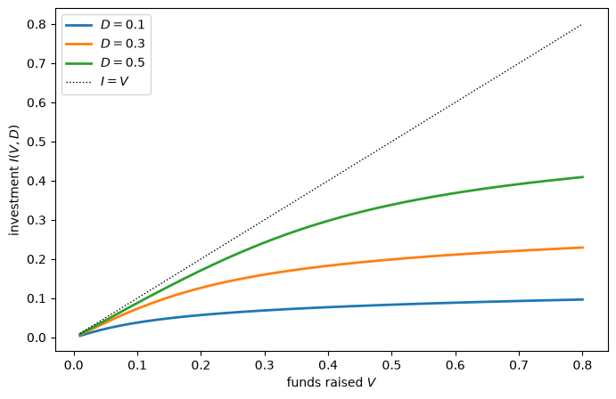
Fig. 56.1 Investment given funds raised and debt#
As Lemma 2 says, investment increases with both \(V\) and \(D\), and the manager always keeps something for perquisites.
56.3. Bonding equilibrium#
Investors do not observe \(I\), but they know \(U\), \(F\), and \(g\), so they can compute the function \(I(V, D)\).
Their perceptions are rational: they value the firm at the expected profit of the investment that the manager will actually choose,
Given \(D\), a bonding equilibrium, which Grossman and Hart also call a precommitment equilibrium, is a pair \((I, V)\) such that \(I\) solves the manager’s problem (56.2) given \((V, D)\), and \(V = g(I)/R\).
If investors offered a \(V\) above \(g(I(V, D))/R\), the firm would be overvalued; if they offered less, it would be undervalued; only when (56.4) holds are investors willing to pay exactly \(V\).
A bonding equilibrium is a fixed point of the kind studied in Rational Expectations Equilibrium.
The manager chooses investment taking as given the funds \(V\) that investors supply.
Those funds rest on investors’ perception of how much the manager will invest.
Equilibrium requires the perception to be correct.
This is analogous to the “big \(K\), little \(k\)” device of Rational Expectations Equilibrium and Investment Under Uncertainty: the manager’s actual investment plays the role of little \(k\), investors’ perception plays the role of big \(K\), and the two are equated only after the manager’s problem has been solved.
Unlike the competitive firms of those lectures, the manager is not small; the manager cannot move investors’ perception by deviating because investors do not observe \(I\).
The function \(g^{-1}(RV)\) on the left of (56.4) is increasing and convex in \(V\), with slope zero at \(V = 0\).
The function \(I(V, D)\) on the right increases with slope between zero and one.
From these properties and \(g'(0) = \infty\), Grossman and Hart conclude, in their Proposition 1:
Proposition (Equilibria for a given level of debt)
For each \(D\), \(V = 0\) solves (56.4), and there is at least one other solution \(V > 0\).
As we show below, a positive solution also needs a condition near \(V = 0\) that the argument leaves implicit, and the proposition can fail.
The solution \(V = 0\) arises because if the market thinks that the firm is worthless, it is worthless: the manager cannot raise any capital.
Bankruptcy is essential for the other solutions.
Without the threat of bankruptcy, the manager’s utility would be just \(U(V - I)\), the manager would set \(I = 0\) for every \(V\), and \(I = V = 0\) would be the only solution.
Although bankruptcy is costly for the manager, it is what lets the manager convince the market that the funds will be invested, and so raise capital.
The argument for a positive solution also needs \(I(V, D)\) to lie above \(g^{-1}(RV)\) for small \(V\).
That need not hold, because a manager who raises little money invests very little of it, so that \(I(V, D)\) also has slope zero at \(V = 0\).
With the functional forms of our example, the first-order condition (56.3) gives \(I(V, D) \approx (\alpha \, r(D) \, V / b)^{1/(1 - \alpha)}\) near \(V = 0\), while \(g^{-1}(RV) = (RV)^{1/\alpha}\).
So near zero, \(I(V, D)\) lies above \(g^{-1}(RV)\) when \(\alpha < 1/2\), does so when \(\alpha = 1/2\) if and only if \(r(D) > 2bR\), and lies below it when \(\alpha > 1/2\).
Because the manager cannot invest more than the funds raised, an equilibrium needs \(g(I)/R = V \ge I\), so equilibrium values of \(I\) and \(V\) are at most the level \(\hat I\) at which \(g(\hat I)/R = \hat I\), which is \(R^{-1/(1 - \alpha)}\) in our example.
Fig. 56.2 plots both sides of (56.4) against \(V\), for our example with \(D = 0.3\) and for a variant with \(g(I) = I^{0.8}\) and \(D = 0.15\).
In each panel, the curve \(g^{-1}(RV)\) is the investment that investors must expect in order to pay \(V\), the curve \(I(V, D)\) is the investment that the manager actually chooses, and the bonding equilibria are the crossings.
def equilibrium_values(D, firm, n=400):
    "Positive solutions V of g^{-1}(R V) = I(V, D), found on a grid of V."
    gap = lambda V: manager_I(V, D, firm) - g_inverse(firm.R * V, firm)
    # positive equilibria have V < I_hat; the grid misses any with V < 1e-4
    grid = np.linspace(1e-4, I_hat(firm) * (1 - 1e-3), n)
    gaps = np.array([gap(V) for V in grid])
    roots = np.flatnonzero(np.sign(gaps[:-1]) != np.sign(gaps[1:]))
    return [brentq(gap, grid[k], grid[k + 1], xtol=1e-14) for k in roots]

firm_08 = create_firm(α=0.8)
examples = [(firm, 0.3, 0.8), (firm_08, 0.15, 0.25)]

fig, axes = plt.subplots(1, 2, figsize=(11, 4.5))
for ax, (firm_i, D, V_max) in zip(axes, examples):
    V_grid = np.linspace(1e-3, V_max, 300)
    I_values = [manager_I(V, D, firm_i) for V in V_grid]
    ax.plot(V_grid, I_values, lw=2, label='$I(V, D)$')
    ax.plot(V_grid, g_inverse(firm_i.R * V_grid, firm_i), lw=2,
            label='$g^{-1}(RV)$')
    for V in equilibrium_values(D, firm_i):
        ax.plot(V, manager_I(V, D, firm_i), 'ko')
    ax.set_title(rf'$\alpha = {firm_i.α}$, $D = {D}$')
    ax.set_xlabel('funds raised $V$')
    ax.set_ylabel('investment')
    ax.legend()
plt.tight_layout()
plt.show()
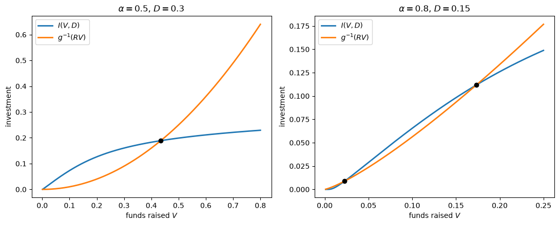
Fig. 56.2 Bonding equilibria at fixed debt#
The left panel has one positive equilibrium and the right panel has two, so the number of equilibria depends on the technology; we explain the counts below, after introducing the debt that sustains a given level of investment.
With several equilibria, Grossman and Hart assume that the manager chooses among them.
Which one the manager prefers is not obvious in general: an equilibrium with a higher \(V\) has more investment and less risk of bankruptcy, but it may leave less for perquisites, \(V - I\).
The next cell computes the manager’s expected utility, \(U(V - I) [1 - F(D - g(I))]\), at the two equilibria in the right panel of Fig. 56.2.
D_08 = 0.15
for V in equilibrium_values(D_08, firm_08):
    I = g_inverse(firm_08.R * V, firm_08)
    p_bankrupt = F(D_08 - g(I, firm_08), firm_08)
    expected_utility = U(V - I, firm_08) * (1 - p_bankrupt)
    print(f"V = {V:.4f}: I = {I:.4f}, perquisites V - I = {V - I:.4f}, "
          f"P(bankruptcy) = {p_bankrupt:.3f}, "
          f"expected utility = {expected_utility:.4f}")
V = 0.0227: I = 0.0088, perquisites V - I = 0.0139, P(bankruptcy) = 0.899, expected utility = 0.0119
V = 0.1733: I = 0.1118, perquisites V - I = 0.0615, P(bankruptcy) = 0.408, expected utility = 0.1468
Here the high-value equilibrium is better for the manager on every count: it brings more perquisites as well as a much lower probability of bankruptcy, and it gives the manager about twelve times the expected utility of the low-value equilibrium.
56.4. Choosing the level of debt#
The manager chooses \(D\), and so chooses among equilibria.
The manager treats \(D\) differently from \(I\): because investors observe \(D\) but not \(I\), investment is chosen taking investors’ valuation \(V\) as given, while debt is chosen taking into account how the equilibrium valuation responds to it, and that is what makes debt a way for the manager to commit.
In the language of Equilibrium Capital Structures with Incomplete Markets, the manager is a price-function taker with respect to \(D\) and a price taker with respect to \(I\); the firm in that lecture is a price-function taker with respect to both of its choices, capital and debt, because investors observe both.
The manager also resembles the Stackelberg leader of Stackelberg Plans, who would like followers to believe a promise about a later action that the leader would not keep if free to reoptimize; here the promise concerns investment, and debt makes it credible.
Analyzing the choice of \(D\) directly is awkward, because the manager’s best equilibrium \(V(D)\) can jump when \(D\) changes.
Grossman and Hart get around the difficulty by treating \(I\), rather than \(D\), as the manager’s choice.
56.4.1. The debt that sustains an investment level#
For each \(I\) between \(0\) and \(\hat I\), Grossman and Hart ask what level of debt \(D(I)\) sustains the equilibrium with investment \(I\) and value \(V = g(I)/R\).
Setting \(V = g(I)/R\) in the first-order condition (56.3) gives
Under Assumption 1, the left side increases with \(D\), so (56.5) has at most one solution \(D(I)\), and Lemma 1 then guarantees that \(I = I(g(I)/R, D(I))\).
\(D(I)\) may be negative, in which case the manager sustains the equilibrium by lending rather than borrowing.
With a normal distribution, the hazard rate takes every positive value, so \(D(I)\) is defined for every \(0 < I < \hat I\).
The function \(D(I)\) explains the counts of equilibria in Fig. 56.2: a debt level \(D\) sustains a positive equilibrium with investment \(I\) exactly when \(D = D(I)\).
Write \(\psi(I)\) for the right side of (56.5), so that \(D(I) = g(I) + r^{-1}(\psi(I))\); since \(r\) is increasing, \(D(I)\) increases everywhere when \(\psi\) does, as Grossman and Hart note.
With our functional forms, \(\psi(I) = b I^{1 - 2\alpha} / [\alpha (1/R - I^{1 - \alpha})]\), which goes to infinity as \(I \to \hat I\), so \(D(I) \to \infty\) there.
In our example, \(\alpha = 1/2\), and \(\psi(I) = 2b / (1/R - \sqrt{I})\) increases from \(2bR = 1\), so \(D(I)\) increases from \(r^{-1}(1) \approx -0.17\): lower levels of debt sustain no positive equilibrium, so Proposition 1 fails for them, and higher levels sustain exactly one.
When \(\alpha < 1/2\), \(\psi(I) \to 0\) as \(I \to 0\), so \(D(I) \to -\infty\), and every level of debt sustains at least one positive equilibrium, as Proposition 1 states.
With \(g(I) = I^{0.8}\), \(\psi(I) \to \infty\) as \(I \to 0\), so \(D(I)\) first falls, to a minimum of about \(0.09\), and then rises: lower levels of debt sustain no positive equilibrium, and higher levels sustain two.
The next cell computes \(D(I)\), checks these thresholds, and counts the positive equilibria for several levels of debt, including a variant with \(\alpha = 0.4\).
def sustaining_debt(I, firm):
    "The debt D(I) that sustains the equilibrium with investment I."
    c = g(I, firm) / firm.R - I
    ψ = U_prime(c, firm) / (U(c, firm) * g_prime(I, firm))
    return g(I, firm) + hazard_inverse(ψ, firm)

D_low = hazard_inverse(2 * firm.b * firm.R, firm)
res = minimize_scalar(lambda I: sustaining_debt(I, firm_08),
                      bounds=(1e-6, I_hat(firm_08) * (1 - 1e-6)),
                      method='bounded')
print(f"α = 0.5: D(I) rises from r^(-1)(2bR) = {D_low:.4f}")
print(f"α = 0.8: D(I) has a minimum of {res.fun:.4f} at I = {res.x:.4f}")

firm_04 = create_firm(α=0.4)
D_small_I = [sustaining_debt(I, firm_04) for I in (1e-4, 1e-8, 1e-12)]
print(f"α = 0.4: D(I) at I = 1e-4, 1e-8, 1e-12: {np.round(D_small_I, 3)}")

cases = ((firm_04, (-0.2, 0.0, 0.3)),
         (firm, (-0.2, -0.1, 0.0, 0.3)),
         (firm_08, (0.05, 0.1, 0.15)))
for firm_i, debt_levels in cases:
    for D in debt_levels:
        V_values = np.round(equilibrium_values(D, firm_i), 4)
        print(f"α = {firm_i.α}, D = {D:5}: positive equilibria {V_values}")
α = 0.5: D(I) rises from r^(-1)(2bR) = -0.1691
α = 0.8: D(I) has a minimum of 0.0924 at I = 0.0349
α = 0.4: D(I) at I = 1e-4, 1e-8, 1e-12: [-0.22  -0.311 -0.366]
α = 0.4, D =  -0.2: positive equilibria [0.0371]
α = 0.4, D =   0.0: positive equilibria [0.1955]
α = 0.4, D =   0.3: positive equilibria [0.4575]
α = 0.5, D =  -0.2: positive equilibria []
α = 0.5, D =  -0.1: positive equilibria [0.0653]
α = 0.5, D =   0.0: positive equilibria [0.1592]
α = 0.5, D =   0.3: positive equilibria [0.4347]
α = 0.8, D =  0.05: positive equilibria []
α = 0.8, D =   0.1: positive equilibria [0.0462 0.0982]
α = 0.8, D =  0.15: positive equilibria [0.0227 0.1733]
With \(\alpha = 0.4\), \(D(I)\) keeps falling as \(I\) shrinks, so every level of debt sustains a positive equilibrium, though for very low debt the equilibrium value \(V\) is too small for our grid to find.
56.4.2. The manager’s problem#
The manager’s problem becomes
Write \(x = D(I) - g(I)\) for the bankruptcy threshold.
Differentiating \(W\) and using (56.5) to replace \(U'/U\) by \(r(x) \, g'(I)\) gives
so the sign of \(W'(I)\) is the sign of \(g'(I)^2/R - D'(I)\), and setting \(W'(I) = 0\) gives Grossman and Hart’s Proposition 2, a necessary condition that several levels of investment can satisfy.
Proposition (The slope of debt at the optimum)
At the manager’s optimal investment level,
Subtracting \(g'(I)\) from both sides, (56.8) says that \(D'(I) - g'(I) = g'(I) \, [g'(I)/R - 1]\).
One more unit of investment raises the manager’s consumption \(g(I)/R - I\) by \(g'(I)/R - 1\), and it raises net liabilities \(D(I) - g(I)\), and with them the risk of bankruptcy, by \(D'(I) - g'(I)\).
By (56.5), \(U'/U = r \, g'\), so the manager is willing to accept \(g'(I)\) more units of net liabilities for one more unit of consumption, and at the optimum the two effects offset.
Lemma 4 of Grossman and Hart [1982] shows that \(D'(I) > g'(I)\) whenever \(I \ge I^\ast\), so that investment beyond \(I^\ast\) raises net liabilities \(D(I) - g(I)\) and with them the probability of bankruptcy.
Grossman and Hart’s Proposition 3 follows.
Proposition (Underinvestment)
The manager’s optimal investment level is below \(I^\ast\).
The reason is simple: if \(I \ge I^\ast\), then \(g'(I)^2/R \le g'(I) < D'(I)\) by Lemma 4, so \(W'(I) < 0\) by (56.7).
A small cut in investment then lowers the probability of bankruptcy, and it does not lower the manager’s consumption \(g(I)/R - I\), which peaks at \(I^\ast\) and so does not rise with \(I\) beyond it.
So the separation of ownership from control leads to underinvestment relative to the classical solution.
56.4.3. The manager’s choice in our example#
The next cell computes the manager’s optimal investment and debt in our example.
def outcomes(I, firm):
    "Sustaining debt, probability of bankruptcy, and expected utility at I."
    D = sustaining_debt(I, firm)
    p_bankrupt = F(D - g(I, firm), firm)
    return D, p_bankrupt, U(g(I, firm) / firm.R - I, firm) * (1 - p_bankrupt)

def manager_welfare(I, firm):
    "The manager's expected utility W(I) in the equilibrium with investment I."
    return outcomes(I, firm)[2]

def optimal_policy(firm):
    "The manager's optimal investment and debt."
    I = minimize_scalar(lambda I: -manager_welfare(I, firm),
                        bounds=(1e-8, I_hat(firm) * (1 - 1e-8)),
                        method='bounded', options={'xatol': 1e-12}).x
    return I, sustaining_debt(I, firm)

def equity_value(I, D, firm):
    "Market value of equity, E max(0, g(I) - D + s) / R."
    m = g(I, firm) - D
    z = m / firm.σ
    return (m * norm.cdf(z) + firm.σ * norm.pdf(z)) / firm.R

I_opt, D_opt = optimal_policy(firm)
V_opt = g(I_opt, firm) / firm.R
V_star = g(I_star(firm), firm) / firm.R
V_e = equity_value(I_opt, D_opt, firm)
h = 1e-6
D_slope = (sustaining_debt(I_opt + h, firm)
           - sustaining_debt(I_opt - h, firm)) / (2 * h)

print(f"investment I = {I_opt:.4f}  (I* = {I_star(firm):.4f})")
print(f"market value V = {V_opt:.4f}  (V* = {V_star:.4f})")
print(f"debt D = {D_opt:.4f}, probability of bankruptcy = "
      f"{F(D_opt - g(I_opt, firm), firm):.4f}")
print(f"value of equity = {V_e:.4f}, value of debt = {V_opt - V_e:.4f}")
print(f"D'(I) = {D_slope:.4f}, "
      f"g'(I)^2 / R = {g_prime(I_opt, firm)**2 / firm.R:.4f}")
print(f"manager's expected utility = {manager_welfare(I_opt, firm):.4f}, "
      f"classical = {U(V_star - I_star(firm), firm):.4f}")
investment I = 0.1995  (I* = 0.2500)
market value V = 0.4467  (V* = 0.5000)
debt D = 0.3134, probability of bankruptcy = 0.0914
value of equity = 0.1375, value of debt = 0.3092
D'(I) = 1.2531, g'(I)^2 / R = 1.2531
manager's expected utility = 0.4517, classical = 0.5000
The manager invests about 20 percent less than the classical level, finances the firm with a mix of debt and equity, and accepts a probability of bankruptcy of about 9 percent.
The last two lines check Proposition 2 and show that the manager would be better off if investment were observable.
We compute the value of equity as \(E \max(0, g(I) - D + s)/R\), which is formula (36) of Grossman and Hart [1982] when \(R = 1\).
The value of debt is the rest of \(V\).
Like Grossman and Hart, we let profit be negative, so creditors bear losses below zero, but at the manager’s choice, with \(\sigma = 0.1\), the probability of negative profit is negligible.
An all-equity firm, with \(D = 0\), can sustain only a small investment.
I_equity = brentq(lambda I: sustaining_debt(I, firm), 1e-8, I_star(firm))
print(f"with D = 0: I = {I_equity:.4f}, V = {g(I_equity, firm) / firm.R:.4f}, "
      f"manager's expected utility = {manager_welfare(I_equity, firm):.4f}")
with D = 0: I = 0.0254, V = 0.1592, manager's expected utility = 0.3455
The all-equity firm is worth just over a third of the firm that the manager chooses, and the manager is worse off.
Even without debt, the firm goes bankrupt when its profit is negative, which happens with a probability of about 6 percent at this investment level, and that threat is what sustains the small investment.
The next cell collects the three cases: the classical solution, in which investors observe \(I\) and the manager never goes bankrupt, the manager’s choice, and the all-equity firm.
rows = [("observable I", I_star(firm), None),
        ("manager's choice", I_opt, D_opt),
        ("all-equity firm", I_equity, 0.0)]
print(f"{'':18s}{'I':>8s}{'V':>8s}{'D':>8s}{'P(bankrupt)':>13s}"
      f"{'utility':>9s}")
for name, I, D in rows:
    V = g(I, firm) / firm.R
    p_bankrupt = 0.0 if D is None else F(D - g(I, firm), firm)
    D_text = '-' if D is None else f"{D:.3f}"
    utility = U(V - I, firm) * (1 - p_bankrupt)
    print(f"{name:18s}{I:8.3f}{V:8.3f}{D_text:>8s}{p_bankrupt:13.3f}"
          f"{utility:9.3f}")
                         I       V       D  P(bankrupt)  utility
observable I         0.250   0.500       -        0.000    0.500
manager's choice     0.200   0.447   0.313        0.091    0.452
all-equity firm      0.025   0.159   0.000        0.056    0.346
Fig. 56.3 shows the debt that sustains each investment level, the probability of bankruptcy that comes with it, and the manager’s expected utility.
I_grid = np.linspace(0.005, 0.6, 200)
values = np.array([outcomes(I, firm) for I in I_grid])
at_choice, at_equity = outcomes(I_opt, firm), outcomes(I_equity, firm)
titles = ['debt $D(I)$', 'probability of bankruptcy',
          "manager's expected utility"]

fig, axes = plt.subplots(1, 3, figsize=(13, 4))
for k, ax in enumerate(axes):
    ax.plot(I_grid, values[:, k], lw=2)
    ax.plot(I_opt, at_choice[k], 'ko', label="manager's choice")
    ax.plot(I_equity, at_equity[k], 'o', mfc='white', mec='k',
            label='all-equity firm')
    ax.axvline(I_star(firm), color='gray', ls=':', lw=1.5, label='$I^*$')
    ax.set_xlabel('investment $I$')
    ax.set_title(titles[k])
axes[0].axhline(0, color='k', lw=0.5)
axes[0].legend()
plt.tight_layout()
plt.show()
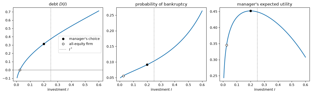
Fig. 56.3 Sustaining debt, bankruptcy, and welfare#
The more the manager wants to invest, the more debt it takes to make the investment credible, and the more likely is bankruptcy.
The manager’s expected utility peaks at an investment level below \(I^\ast\), as Proposition 3 says.
Fig. 56.4 shows the same choice as a menu.
Each bonding equilibrium offers the manager perquisites \(c = g(I)/R - I\) and a probability \(1 - F(D(I) - g(I))\) of keeping the job, and the manager picks the point on the menu that reaches the highest indifference curve of \(U(c) \, [1 - F(x)]\).
I_path = np.linspace(0.002, 0.5, 400)
c_path = g(I_path, firm) / firm.R - I_path
keep_path = [1 - outcomes(I, firm)[1] for I in I_path]
c_grid = np.linspace(0.12, 0.26, 200)
W_opt = manager_welfare(I_opt, firm)
I_s = I_star(firm)

fig, ax = plt.subplots(figsize=(8, 5))
ax.plot(c_path, keep_path, lw=2, label='bonding equilibria')
for W_level, ls in ((0.42, ':'), (W_opt, '-'), (0.47, ':')):
    ax.plot(c_grid, W_level / U(c_grid, firm), color='k', ls=ls, lw=1)
ax.plot(V_opt - I_opt, 1 - outcomes(I_opt, firm)[1], 'ko',
        label="manager's choice")
ax.plot(V_star - I_s, 1 - outcomes(I_s, firm)[1], 'o', mfc='white',
        mec='k', label='$I = I^*$')
ax.set_xlim(0.12, 0.26)
ax.set_ylim(0.75, 1.0)
ax.set_xlabel('perquisites $g(I)/R - I$')
ax.set_ylabel('probability of keeping the job')
ax.legend(loc='lower left')
plt.show()
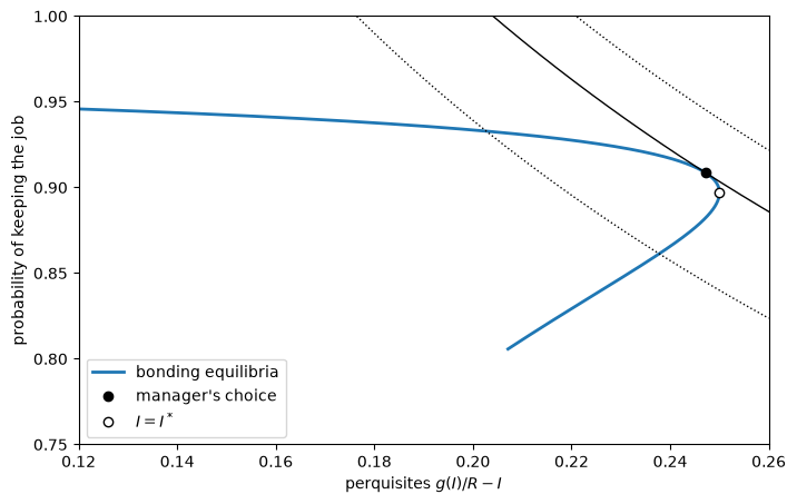
Fig. 56.4 Perquisites and job retention#
The black curves are indifference curves of the manager, and the solid one is the highest that the menu reaches.
Perquisites are largest at \(I^\ast\), where the menu bends back, so the highest indifference curve touches the menu on its upper branch, at an investment level below \(I^\ast\), as Proposition 3 says.
The tangency is Proposition 2: along the menu, the manager’s indifference curves trade \(g'(I)\) units of net liabilities for one unit of perquisites, and the menu’s own rate is \([D'(I) - g'(I)] / [g'(I)/R - 1]\).
The figure also shows where the manager’s loss relative to the classical solution comes from.
Because perquisites are flat near \(I^\ast\), cutting investment by 20 percent lowers them only from \(0.25\) to about \(0.247\), and almost all of the fall in expected utility, from \(0.5\) to \(0.45\), comes from the 9 percent risk of bankruptcy.
56.4.4. Market value and debt#
Fig. 56.5 plots the same equilibria in another way.
As \(I\) ranges between \(0\) and \(\hat I\), each equilibrium is a pair of debt \(D(I)\) and market value \(V = g(I)/R\), and \(V = 0\) is an equilibrium at every level of debt.
The figure shows these pairs for our example and for the variant with \(g(I) = I^{0.8}\), together with the classical value \(V^\ast = g(I^\ast)/R\).
fig, axes = plt.subplots(1, 2, figsize=(11, 4.5))
for ax, firm_i in zip(axes, (firm, firm_08)):
    I_path = np.linspace(1e-4, I_hat(firm_i) * (1 - 1e-3), 400)
    D_path = [sustaining_debt(I, firm_i) for I in I_path]
    ax.axhline(0, color='C1', lw=1, ls='--', label='equilibrium $V = 0$')
    ax.plot(D_path, g(I_path, firm_i) / firm_i.R, color='C0', lw=2,
            label='positive equilibria')
    ax.axhline(g(I_star(firm_i), firm_i) / firm_i.R, color='gray', ls=':',
               lw=1.5, label='classical value $V^*$')
    I_i, D_i = optimal_policy(firm_i)
    ax.plot(D_i, g(I_i, firm_i) / firm_i.R, 'ko', label="manager's choice")
    ax.set_xlim(-0.3, 1.0)
    ax.set_ylim(-0.03, 1.0)
    ax.set_title(rf'$\alpha = {firm_i.α}$')
    ax.set_xlabel('debt $D$')
    ax.set_ylabel('market value $V$')
axes[0].plot(0, g(I_equity, firm) / firm.R, 'o', mfc='white', mec='k',
             label='all-equity firm')
for ax in axes:
    ax.legend(loc='upper left')
plt.tight_layout()
plt.show()
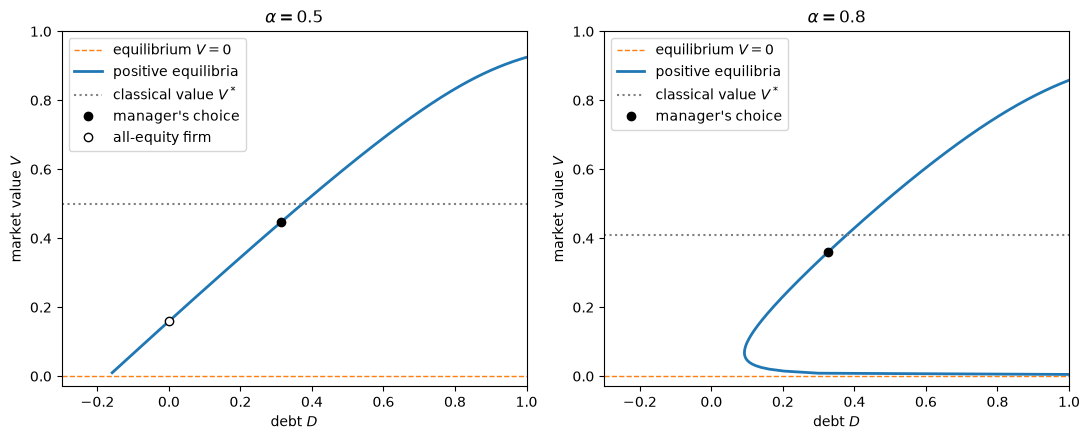
Fig. 56.5 Market value and debt#
If investors could observe \(I\), the firm would be worth \(V^\ast\) whatever its debt, as the Modigliani-Miller theorem says.
In a bonding equilibrium, by contrast, the firm’s market value depends on its debt.
In the left panel, there is one positive equilibrium for each debt level above about \(-0.17\), and market value rises with debt.
To the right of \(D(I^\ast) \approx 0.37\), more debt would push investment above \(I^\ast\) and market value above \(V^\ast\), but the manager’s perquisites would fall and bankruptcy would become more likely, so the manager chooses less debt.
In the right panel, the curve bends back at \(D \approx 0.09\): lower debt sustains only \(V = 0\), so an all-equity firm cannot raise capital, while higher debt sustains two positive equilibria.
On the lower branch, which runs just above \(V = 0\), market value falls as debt rises; the manager’s choice lies on the upper branch, where market value rises with debt.
56.5. Comparative statics#
Comparative statics are hard in this model, because a change in a parameter changes both the manager’s response to a given level of debt and the level of debt needed to sustain a given investment.
Grossman and Hart derive sufficient conditions in their Propositions 4 to 7, which work through the slope of the sustaining debt function.
Their Proposition 4 follows from (56.7).
Proposition (A criterion for comparative statics)
Suppose that the manager’s optimal investment level is a unique and regular maximum of (56.6), so that \(D''(I) - 2 g'(I) g''(I)/R > 0\) there.
If a change in a parameter \(t\) raises \(D'(I) - g'(I)^2/R\) at the optimal investment level, it lowers investment, and if it lowers \(D'(I) - g'(I)^2/R\), it raises investment.
By (56.7), a change that raises \(D'(I) - g'(I)^2/R\) at the old optimum makes \(W'(I)\) negative there, so the manager gains by investing less.
56.5.1. Riskier projects#
Proposition 5 says that a change in the distribution of \(s\) raises investment if it raises the slope of the hazard rate at the bankruptcy threshold, holding fixed the hazard rate itself.
Grossman and Hart show that, by this criterion, a more variable shock lowers investment when \(s\) has a double exponential distribution, and leaves it unchanged locally when \(s\) is uniform.
For a normal distribution with standard deviation \(\sigma\), recall that \(r(x) = \lambda(x/\sigma)/\sigma\), where \(\lambda\) is the hazard rate of the standard normal distribution.
Holding \(r(x) = \rho\) fixed requires \(\lambda(z) = \rho \sigma\), so the standardized threshold \(z = x / \sigma\) rises with \(\sigma\), and the slope \(r'(x) = \lambda'(z)/\sigma^2 = \rho \, [\lambda(z) - z] / \sigma\) falls, because \(\lambda' < 1\).
So by Proposition 5, a larger \(\sigma\) lowers investment.
Proposition 6 gives conditions under which a riskier project also raises the value of equity and lowers the value of debt: the change is a mean-preserving spread, it lowers investment by the criterion of Proposition 5, and it raises the hazard rate at the bankruptcy threshold, holding the threshold fixed.
For a normal distribution, a larger \(\sigma\) satisfies the first two conditions, as we just saw, and the third holds exactly when the standardized bankruptcy threshold \(x / \sigma\) is below about \(-0.84\), that is, when the probability of bankruptcy is below about 20 percent, which in our example is when \(\sigma\) is below about \(0.22\).
Fig. 56.6 shows the comparative statics in our example.
σ_grid = np.linspace(0.01, 0.4, 40)
results = []
for σ in σ_grid:
    firm_σ = create_firm(σ=σ)
    I, D = optimal_policy(firm_σ)
    results.append([I, D, F(D - g(I, firm_σ), firm_σ),
                    equity_value(I, D, firm_σ), g(I, firm_σ) / firm_σ.R])
I_σ, D_σ, p_σ, E_σ, V_σ = np.array(results).T

fig, axes = plt.subplots(2, 2, figsize=(11, 8), sharex=True)
axes[0, 0].plot(σ_grid, I_σ, lw=2)
axes[0, 0].axhline(I_star(firm), color='gray', ls=':', lw=1.5, label='$I^*$')
axes[0, 0].set_title('optimal investment $I$')
axes[0, 0].legend()
axes[0, 1].plot(σ_grid, D_σ, lw=2)
axes[0, 1].set_title('face value of debt $D$')
axes[1, 0].plot(σ_grid, p_σ, lw=2)
axes[1, 0].set_title('probability of bankruptcy')
axes[1, 1].plot(σ_grid, V_σ, 'k', lw=2, label='firm')
axes[1, 1].plot(σ_grid, E_σ, lw=2, label='equity')
axes[1, 1].plot(σ_grid, V_σ - E_σ, lw=2, label='debt')
axes[1, 1].set_title('market values')
axes[1, 1].legend()
for ax in axes[1]:
    ax.set_xlabel(r'standard deviation of profits $\sigma$')
plt.tight_layout()
plt.show()
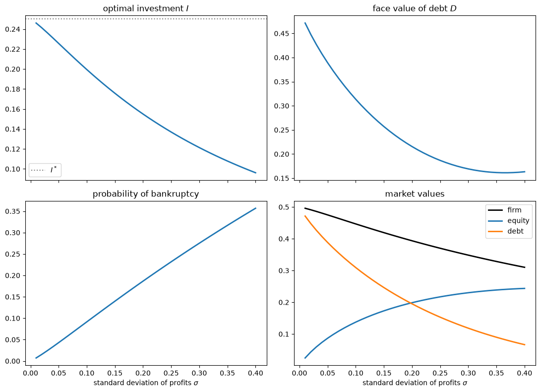
Fig. 56.6 The manager’s choices and profit risk#
As \(\sigma\) rises, the manager invests less and goes bankrupt more often, and the firm is financed more with equity and less with debt.
The market value of debt falls throughout, while the face value \(D\) falls until \(\sigma\) is about \(0.37\) and then edges up, echoing Grossman and Hart’s observation that in their uniform example debt is not monotone in the spread of \(s\).
Equity becomes more valuable and debt less valuable even beyond the range in which Proposition 6 applies.
So across firms that differ only in \(\sigma\), market value and the debt-equity ratio rise and fall together, which is Grossman and Hart’s example of how the bonding theory can produce the cross-section relation that signaling theories predict; we return to this point in the discussion below.
For the larger values of \(\sigma\), the probability of negative profit is no longer negligible, about 2.5 percent at \(\sigma = 0.2\) and 22 percent at \(\sigma = 0.4\), so part of the fall in the value of debt reflects creditors bearing losses below zero.
56.5.2. No uncertainty#
As \(\sigma \to 0\), investment approaches \(I^\ast\) and debt approaches \(g(I^\ast)\).
Section 4.5 of Grossman and Hart [1982] explains why.
Without uncertainty, the manager loses everything whenever \(g(I) < D\), so the manager sets \(g(I) = D\), and the firm’s value is \(V(D) = D/R\).
The manager then maximizes \(U(D/R - g^{-1}(D))\), which gives \(g'(I) = R\), so the manager maximizes the net market value of the firm.
The firm borrows \(g(I^\ast)/R\), its equity is worthless, and the manager, who keeps the residual \(V - I^\ast\), is in effect its owner.
Uncertainty is what makes equity valuable: with a random \(s\), the manager reduces debt to the point where there are states in which \(g(I) + s > D\).
Grossman and Hart caution that in the certainty case, the same outcome could be achieved with all-equity finance and a rule that fires the manager unless profit reaches \(g(I^\ast)\).
56.5.3. More risk aversion#
Proposition 7 of Grossman and Hart [1982] states that replacing \(U\) by \(U^a\) with \(a < 1\), which makes the manager more risk averse, lowers investment.
In our example, replacing \(U(c) = c^b\) by \(U^a\) amounts to replacing \(b\) by \(ab\), so we can check the proposition by varying \(b\).
The coefficient of relative risk aversion of \(c^b\) is \(1 - b\), and Fig. 56.7 plots the manager’s choices against it, so that more risk-averse managers are to the right.
b_grid = np.linspace(0.1, 0.9, 17)
results = []
for b in b_grid:
    firm_b = create_firm(b=b)
    I, D = optimal_policy(firm_b)
    results.append([I, D, F(D - g(I, firm_b), firm_b)])
results = np.array(results)

labels = ['optimal investment $I$', 'debt $D$', 'probability of bankruptcy']
fig, axes = plt.subplots(1, 3, figsize=(13, 4))
for k, ax in enumerate(axes):
    ax.plot(1 - b_grid, results[:, k], lw=2)
    ax.set_title(labels[k])
    ax.set_xlabel('relative risk aversion $1 - b$')
plt.tight_layout()
plt.show()
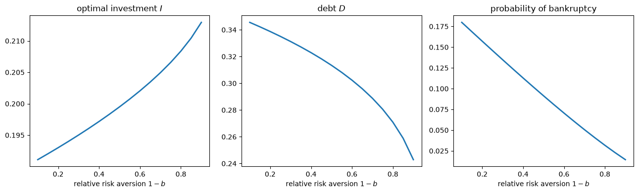
Fig. 56.7 The manager’s choices and risk aversion#
In our example, a more risk-averse manager invests more, the opposite of what Proposition 7 states, although the effect is small: investment rises only from about 0.191 to 0.213 as relative risk aversion rises from \(0.1\) to \(0.9\).
The more risk-averse manager also borrows less and goes bankrupt less often: with relative risk aversion \(0.9\), the probability of bankruptcy is about 1.4 percent, against 18 percent with relative risk aversion \(0.1\).
A lower \(b\) makes \(U'/U = b/c\) smaller, so the manager values extra perquisites less relative to the utility at stake in bankruptcy, the right side of (56.5) falls, and less debt sustains any given level of investment.
This direct effect outweighs the extra debt that the higher investment requires, so debt falls, from about \(0.35\) to \(0.24\) as relative risk aversion rises from \(0.1\) to \(0.9\).
The effect of risk aversion turns out to depend on the shape of the hazard rate.
Recall that \(\psi(I)\) is the right side of (56.5).
Replacing \(U\) by \(U^a\) multiplies \(U'/U\) by \(a\), so with \(U^a\) the right side is \(a \psi(I)\), and the bankruptcy threshold \(x = D(I) - g(I)\) solves \(r(x) = a \psi(I)\).
Taking logs, \(\log r(x) = \log a + \log \psi(I)\), and differentiating with respect to \(I\) gives
At the optimum, \(D'(I) = g'(I)^2/R > g'(I)\) because \(I < I^\ast\), so \((\log \psi)'(I) > 0\).
More risk aversion lowers the hazard rate needed to sustain every level of investment in the same proportion, so \(a\) affects the right side only through the threshold \(x\), which rises with \(a\) at the rate \(dx/da = \psi(I)/r'(x)\).
So
which has the sign of \(-(\log r)''(x)\).
Grossman and Hart write the slope in the equivalent form \(a \psi'(I)/r'(x)\) and hold \(r'(x)\) fixed as \(a\) changes, which leaves only the explicit factor \(a\) and gives \(\partial [D'(I) - g'(I)^2/R]/\partial a = \psi'(I)/r'(x) > 0\); by Proposition 4, that would mean that a lower \(a\) raises investment, the opposite of the sign stated in Proposition 7.
The log form shows that the explicit factor \(a\) cancels against \(r(x) = a \psi(I)\), so the whole effect runs through the threshold.
So more risk aversion raises investment when the log of the hazard rate is concave at the bankruptcy threshold, lowers it when the log of the hazard rate is convex, and leaves it unchanged when the log of the hazard rate is linear.
The sign stated in Proposition 7 is therefore right for hazard rates whose logs are convex, such as the uniform hazard rate \(1/(\bar s - x)\) of their appendix and the double exponential hazard rate below zero, for which the term that Grossman and Hart omit reverses the sign of the term they keep.
The log of the normal hazard rate is concave everywhere, since \((\log \lambda)'' = \lambda' - 1 < 0\), so in our example more risk aversion raises investment.
When the log of the hazard rate is linear, risk aversion has no effect on investment at all, not just locally.
For the Gumbel distribution for minima, \(F(x) = 1 - \exp(-e^{(x - m)/\beta})\), with \(m\) chosen so that \(s\) has mean zero, the hazard rate is \(r(x) = e^{(x - m)/\beta}/\beta\), so that \(1 - F(x) = e^{-\beta r(x)}\).
Along bonding equilibria, (56.5) then gives
and replacing \(U\) by \(U^a\) replaces \(W\) by \(W^a\), which leaves the optimal investment unchanged; only the debt that sustains it changes.
Exercise 56.1 asks you to verify that, in the uniform example, more risk aversion lowers investment when the optimum lies on the branch of \(D(I)\) that solves (56.5), and to see what happens on the other branches, where Propositions 4 to 7 do not apply.
56.6. Takeovers#
56.6.1. The free-rider problem#
In their earlier paper, Grossman and Hart [1980] asked whether the threat of a takeover bid can discipline the managers of a widely held corporation.
The usual argument is that if a corporation is badly run, a raider can buy it at a low price, run it well, and sell it at a high price.
Grossman and Hart show that this argument is wrong.
Suppose that the firm’s value is \(q\) under current management and \(v > q\) under the raider, and that the raider offers to buy shares at a price \(p\), which shareholders accept by tendering their shares.
Each shareholder is too small to affect whether the bid succeeds, so a shareholder who expects the bid to succeed compares \(p\) with the value \(v\) of a share in the improved firm and does not tender unless \(p \ge v\).
But at \(p \ge v\), the raider makes no profit, and with any cost of making the bid, the raider loses money.
Shareholders free ride on the raider’s improvement of the firm, and no raids take place, however badly the firm is run.
The remedy that Grossman and Hart propose is a corporate charter that lets a successful raider dilute the property rights of shareholders who do not tender, by up to \(\phi\) dollars, for example by selling the firm’s assets or output on favorable terms to another company that the raider owns.
Then a shareholder who does not tender expects only \(v - \phi\).
Grossman and Hart also rule out bids below the status quo value \(q\), which fail if shareholders expect them to fail, so the lowest tender price at which the bid succeeds is \(p = \max(v - \phi, q)\), and the raider’s profit, if the bid costs \(\xi\), is
A raid occurs when this is positive.
If \(v\) or \(\xi\) is random, the probability of a raid, \(\pi(\phi, q)\), does not rise with the firm’s status quo value \(q\), so a manager who enjoys \(u(q)\) unless the firm is raided chooses \(q\) to maximize \(u(q) \, [1 - \pi(\phi, q)]\).
Here \(u(q)\) is the manager’s utility from running the firm so that it earns profit \(q\), not the utility of consumption \(U\) of the main model; it reflects the manager’s salary, effort, and perquisites, so it need not increase with \(q\).
More dilution makes raids easier and induces the manager to run the firm better, but it also lowers the tender price that shareholders receive when a raid occurs.
So the initial shareholders who write the charter may limit dilution.
Society, which does not care how the gains from a raid are divided, does at least as well with unlimited dilution as with any limit, provided that the amount invested does not depend on shareholders’ returns and that managers’ welfare is ignored (Proposition 5 of Grossman and Hart [1980]).
The divergence arises because there is a single raider: with perfect competition among raiders and no sunk costs of a raid, the raider’s profit is zero, and shareholders themselves choose unlimited dilution.
When investment does depend on shareholders’ returns, society may want to limit dilution too, but never by more than shareholders do (Proposition 6 of Grossman and Hart [1980]).
Exercise 56.2 asks you to compute these choices in an example.
56.6.2. The takeover threat and debt#
Section 4.5 of Grossman and Hart [1982] combines the two disciplines.
Suppose that the manager has a fixed amount \(K\) of capital, raised in the past, to divide between investment \(I\) and perquisites \(K - I\).
The manager enjoys \(U(K - I)\) only if the firm is neither bankrupt nor taken over, and, as in Grossman and Hart [1980], the probability \(\kappa(V)\) that the firm is not taken over increases with its market value \(V = g(I)/R\).
In the notation of the previous subsection, \(\kappa(V) = 1 - \pi(\phi, V)\), with the firm’s market value as its status quo value.
Given \((V, D)\), the manager chooses \(I\) to maximize
Because \(\kappa(V)\) enters multiplicatively and the manager takes investors’ valuation \(V\) as given, it does not affect the manager’s choice of \(I\) given \((V, D)\); Grossman and Hart justify this by assuming that a raider can reverse the manager’s investment, so that the firm’s worth to a raider does not depend on what current management does.
But \(\kappa(V)\) does affect the manager’s expected utility, so the manager chooses \(D\) to raise \(I\) and \(V\) and so reduce the probability of a takeover.
Since the manager’s choice of \(I\) no longer depends on \(V\), each level of debt sustains a single equilibrium; the multiple equilibria of the main model come from the link between \(V\) and perquisites.
Without bankruptcy penalties, \(I\) would not depend on \(D\), and debt could affect neither \(V\) nor the probability of a takeover.
Exercise 56.3 asks you to compute this extension.
56.7. Discussion#
Grossman and Hart contrast their theory with three other explanations of debt.
Early explanations relaxed the Modigliani-Miller assumptions of no bankruptcy and no taxes.
Stiglitz [1974] and Jensen and Meckling [1976] study an entrepreneur who finances a project by selling shares and so retains less than all of the gains from effort, a weakening of incentives that debt largely avoids.
Ross [1977] and Leland and Pyle [1977] explain debt as a signal of a firm’s exogenous quality.
Unlike the entrepreneur of the second explanation, the manager in Grossman and Hart [1982] owns essentially none of the firm, and the incentive comes entirely from the threat of losing the job in bankruptcy, so bankruptcy penalties are crucial.
Ross’s signaling theory predicts that market value and the debt-equity ratio are positively related across firms.
The bonding theory makes no such prediction without further assumptions, because the cross-section relation depends on how firms’ production functions, interest rates, and managers’ tastes are distributed.
Fig. 56.8 illustrates this with two cross sections of firms computed from our example.
def value_and_leverage(firm):
    "Market value and the ratio of the market values of debt and equity."
    I, D = optimal_policy(firm)
    V = g(I, firm) / firm.R
    V_e = equity_value(I, D, firm)
    return V, (V - V_e) / V_e

cross_sections = [
    ([create_firm(σ=σ) for σ in np.linspace(0.05, 0.2, 16)],
     r'firms differ in $\sigma$'),
    ([create_firm(b=b) for b in np.linspace(0.2, 0.8, 16)],
     r'firms differ in $b$')]

fig, axes = plt.subplots(1, 2, figsize=(11, 4.5))
for ax, (firms, title) in zip(axes, cross_sections):
    V_values, ratios = np.array([value_and_leverage(f) for f in firms]).T
    ax.plot(V_values, ratios, 'o-', lw=2)
    ax.set_title(title)
    ax.set_xlabel('market value $V$')
    ax.set_ylabel('debt-equity ratio')
plt.tight_layout()
plt.show()
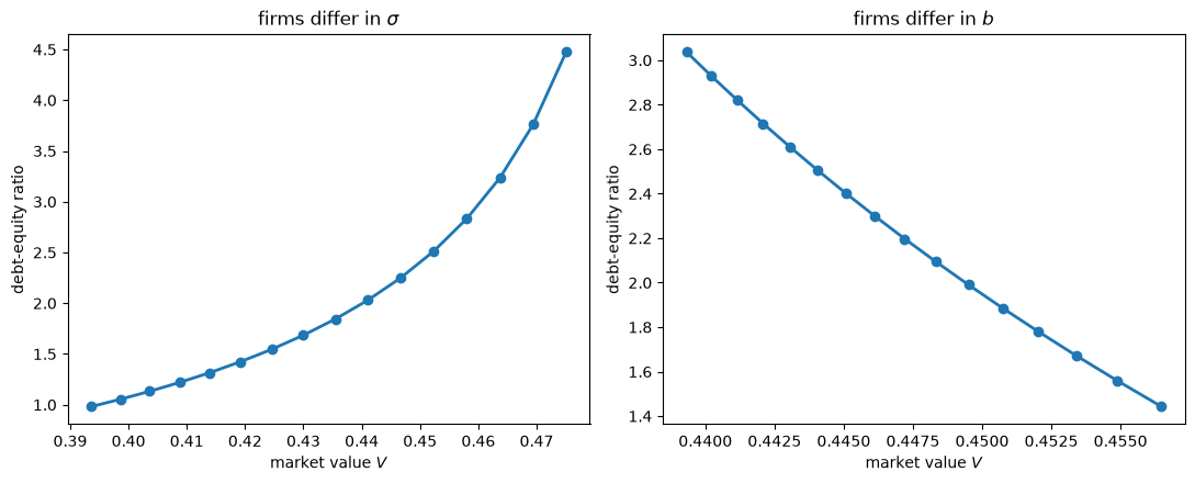
Fig. 56.8 Market value and leverage across firms#
In the left panel, firms differ only in the standard deviation \(\sigma\) of profits, and, as in Fig. 56.6, firms with higher market values have higher debt-equity ratios, as in Ross’s theory.
In the right panel, firms differ only in the manager’s taste parameter \(b\), and firms with higher market values have lower debt-equity ratios, because a more risk-averse manager invests more and borrows less.
Grossman and Hart also note that the manager must receive some surplus from the job for the threat of losing it to be an effective incentive, and that bankruptcy and takeovers have an advantage over salary incentive schemes: they transfer control over information away from current management.
In a comment on the paper, Leland [1982] interpreted the model as a principal-agent problem in which the manager’s reward is \(V - I\) if the firm repays its debt and zero otherwise.
Leland compared bonding to Odysseus, who had himself tied to the mast so that his crew would sail within earshot of the Sirens.
Leland pointed out that if the firm’s true future value were observable by everyone, the same incentive could be provided without debt, by a manager’s promise to resign if the firm’s future value fell short of a target, which might be preferable because it would avoid possible costs of bankruptcy.
In that case, richer contracts, such as stock options, would most likely be preferred.
When both the repayment of debt and the future market value carry information about the firm’s true value, Leland argued, the best contract combines bankruptcy penalties with stock-based rewards, which is what managerial compensation looks like in practice.
In Grossman and Hart’s model bankruptcy has no deadweight cost, so debt and a promise to resign unless profit reaches \(D\) give the same outcome; Exercise 56.4 shows that when profit is publicly observed and dismissal is the only penalty, such a threshold rule is the best one.
The bonding theory is most compelling, Leland argued, when only the manager can observe the firm’s true value, so that the only verifiable event is whether the firm repays its debt.
Leland also noted that debt can still signal: all managers may want some debt to show their honest intentions, but managers of firms with better prospects will be willing to take on more.
56.8. Connections to other lectures#
In A Competitive Entrepreneurial Model of a Stock Market, free entry delivers the Modigliani-Miller theorem; here the separation of ownership from control makes the production plan depend on the financial structure, and the theorem fails.
Irrelevance of Capital Structures with Complete Markets and Equilibrium Capital Structures with Incomplete Markets study firms that choose capital and debt to maximize market value, with default when markets are incomplete; here the firm’s choices serve the manager instead.
Repeated Moral Hazard studies a principal-agent problem with unobserved effort, in which a planner designs incentives; here the manager, who is the agent, sets up the incentives by choosing the firm’s debt.
Rational Expectations Equilibrium and Investment Under Uncertainty explain the “big \(K\), little \(k\)” device, to which a bonding equilibrium is analogous.
56.9. Exercises#
Exercise 56.1
The appendix of Grossman and Hart [1982] studies the case \(g(I) = I^{1/2}\), \(U(c) = c^b\), \(R = 1\), and \(s\) uniformly distributed on \([-\bar s, \bar s]\), so that \(I^\ast = 1/4\).
The uniform hazard rate, \(r(x) = 1/(\bar s - x)\) for \(-\bar s \le x < \bar s\), is increasing only on the support of \(s\), and Grossman and Hart show that the smallest debt that sustains the investment level \(I\) is
where the first expression solves (56.5) and the second puts the bankruptcy threshold at the bottom of the support.
They find that the optimal \(I^{1/2}\) is \(1/2\) when \(\bar s \le 1/(8b)\), is \(1 - 4 b \bar s\) when \(1/(8b) \le \bar s \le (b + 1) / [4b(2b + 1)]\), and is \(b / (2b + 1)\) for larger \(\bar s\).
For \(b = 1/2\), maximize the manager’s expected utility (56.6) numerically for a grid of values of \(\bar s\), and compare the result with Grossman and Hart’s formula.
Plot the optimal \(I^{1/2}\) and \(D\) against \(2 \bar s\), and compute the probability of bankruptcy.
Plot the optimal \(I^{1/2}\) against \(\bar s\) for \(b = 1/4\) and \(b = 1/2\), and relate the result to the discussion of Proposition 7 in the lecture.
Solution
def uniform_debt(I, b, s_bar):
    "Smallest debt that sustains investment I when s is uniform."
    sqrt_I = np.sqrt(I)
    on_foc = ((2 * b + 1) * sqrt_I - 1 + 2 * b * s_bar) / (2 * b)
    return np.maximum(on_foc, sqrt_I - s_bar)

def uniform_welfare(I, b, s_bar):
    "The manager's expected utility at investment I when s is uniform."
    sqrt_I = np.sqrt(I)
    x = uniform_debt(I, b, s_bar) - sqrt_I
    prob_bankrupt = np.clip((x + s_bar) / (2 * s_bar), 0, 1)
    return (sqrt_I - I)**b * (1 - prob_bankrupt)

def uniform_optimum(b, s_bar):
    "Grid search over sqrt(I), then a local refinement."
    grid = np.linspace(1e-4, 1 - 1e-4, 20001)
    k = np.argmax(uniform_welfare(grid**2, b, s_bar))
    lo, hi = grid[max(k - 1, 0)], grid[min(k + 1, len(grid) - 1)]
    sqrt_I = minimize_scalar(lambda z: -uniform_welfare(z**2, b, s_bar),
                             bounds=(lo, hi), method='bounded',
                             options={'xatol': 1e-12}).x
    return sqrt_I**2

def formula_sqrt_I(b, s_bar):
    "Grossman and Hart's closed form for the optimal sqrt(I)."
    if s_bar <= 1 / (8 * b):
        return 0.5
    if s_bar <= (b + 1) / (4 * b * (2 * b + 1)):
        return 1 - 4 * b * s_bar
    return b / (2 * b + 1)

b = 0.5
s_grid = np.linspace(0.01, 0.6, 60)
I_num = np.array([uniform_optimum(b, s) for s in s_grid])
D_num = uniform_debt(I_num, b, s_grid)
x_num = D_num - np.sqrt(I_num)
prob_bankrupt = np.clip((x_num + s_grid) / (2 * s_grid), 0, 1)
formula = np.array([formula_sqrt_I(b, s) for s in s_grid])
gap = np.max(np.abs(np.sqrt(I_num) - formula))
print(f"largest gap between numerical and analytical sqrt(I): {gap:.2e}")

fig, axes = plt.subplots(1, 3, figsize=(13, 4))
axes[0].plot(2 * s_grid, np.sqrt(I_num), lw=2)
axes[0].set_ylabel(r'optimal $I^{1/2}$')
axes[1].plot(2 * s_grid, D_num, lw=2)
axes[1].set_ylabel('optimal debt $D$')
axes[2].plot(2 * s_grid, prob_bankrupt, lw=2)
axes[2].set_ylabel('probability of bankruptcy')
for ax in axes:
    ax.set_xlabel(r'$2 \bar s$')
plt.tight_layout()
plt.show()
largest gap between numerical and analytical sqrt(I): 4.90e-09
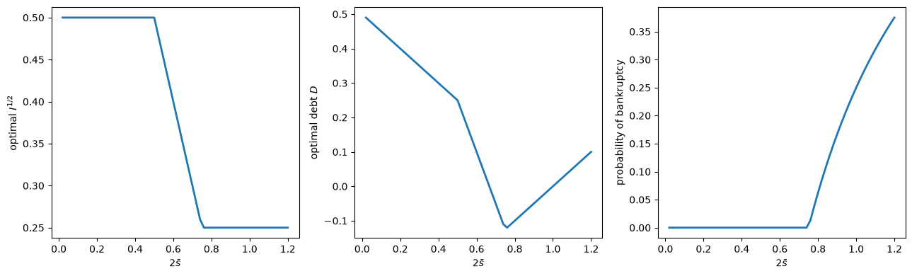
The numerical optimum matches Grossman and Hart’s formula, and the first two panels reproduce their figure 4.A.2, for \(b = 1/2\); the third adds the probability of bankruptcy.
When \(\bar s\) is small, the manager invests \(I^\ast\) and sets \(D = 1/2 - \bar s\), so the firm never goes bankrupt: the hazard rate at the bottom of the support, \(1/(2\bar s)\), is so high that the threat of bankruptcy at the margin disciplines the manager without bankruptcy ever happening.
As \(\bar s\) grows, investment falls, first along \(I^{1/2} = 1 - 4 b \bar s\), still without bankruptcy, and then to the constant \(I^{1/2} = b/(2b + 1)\), with a positive probability of bankruptcy.
Debt is not monotone in \(\bar s\), and as \(\bar s \to 0\), \(I \to I^\ast\) and \(D \to g(I^\ast)\), as in the certainty case of the lecture.
In the third region, where the optimum lies on the branch of \(D(I)\) that solves (56.5), investment does not depend on \(\bar s\), which is what Proposition 5 implies for the uniform case.
s_grid = np.linspace(0.01, 1.0, 100)
fig, ax = plt.subplots(figsize=(8, 5))
for b in (0.25, 0.5):
    sqrt_I = [np.sqrt(uniform_optimum(b, s)) for s in s_grid]
    ax.plot(s_grid, sqrt_I, lw=2, label=f'$b = {b}$')
for s_line in (1/4, 3/4, 5/6):
    ax.axvline(s_line, color='gray', ls=':', lw=1)
ax.set_xlabel(r'$\bar s$')
ax.set_ylabel(r'optimal $I^{1/2}$')
ax.legend()
plt.show()
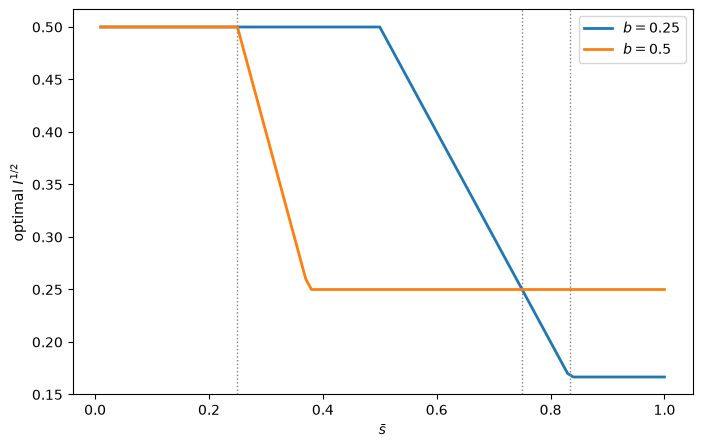
The dotted lines mark \(\bar s = 1/4\), \(3/4\), and \(5/6\).
When \(\bar s > 5/6\), both managers are in the third region, where the optimum lies on the branch of \(D(I)\) that solves (56.5), and the more risk-averse manager, with \(b = 1/4\), invests less, \(I = (b / (2b + 1))^2\), as Proposition 7 states and as the lecture’s analysis predicts for a hazard rate whose log is convex.
For smaller \(\bar s\), at least one manager’s bankruptcy threshold sits at the bottom of the support, either on the branch \(I^{1/2} - \bar s\) of \(D(I)\) (the first region) or at the kink where the two branches meet (the second region), so (56.5) does not hold and Propositions 4 to 7 do not apply.
For \(1/4 < \bar s < 3/4\), the more risk-averse manager invests more: this manager stays at \(I^\ast\) until \(\bar s = 1/(8b) = 1/2\) rather than \(1/4\), and then \(I^{1/2} = 1 - 4 b \bar s\) falls more slowly.
For \(3/4 < \bar s < 5/6\), the more risk-averse manager is still at the kink between the two branches of \(D(I)\) but invests less.
With \(U(c) = c^b\), a lower \(b\) makes \(U'/U = b/c\) smaller, so the manager values extra perquisites less relative to the utility at stake in bankruptcy, and the high hazard rate \(1/(2\bar s)\) at the bottom of the support can sustain more investment.
Exercise 56.2
Consider the model of dilution of Grossman and Hart [1980].
The firm is worth \(v = 1\) to a raider, and the raider’s cost \(\xi\) is uniformly distributed on \([0, 1]\), so that the probability of a raid when the status quo value is \(q \in [0, 1]\) is \(\pi(\phi, q) = \min(\phi, 1 - q)\).
The manager’s utility is \(u(q) = \exp[-\eta (q - 1/2)^2]\), so that, absent any threat of a raid, the manager would choose \(q^\ast = 1/2\), and \(\eta\) measures how costly it is for the manager to depart from \(q^\ast\), so that a larger \(\eta\) makes the manager less responsive to the threat of a raid.
Given \(\phi\), the manager chooses \(q\) to maximize \(u(q) [1 - \pi(\phi, q)]\), choosing the higher \(q\) when indifferent.
Shareholders’ expected return is
and society’s is \(w(\phi)\) plus the raider’s expected profit, \(E[\min(\phi, v - q) - \xi \mid \text{raid}] \, \pi(\phi, q)\).
For \(\eta = 5\) and \(\eta = 20\), compute \(q(\phi)\), \(w(\phi)\), and society’s return on a grid of \(\phi\) between \(0\) and \(1.2\).
Find the shareholders’ preferred \(\phi\) in each case and relate it to Proposition 3 of Grossman and Hart [1980].
Which \(\phi\) does society prefer?
Solution
def raid_prob(φ, q, v=1.0):
    "Probability of a raid when the cost ξ is uniform on [0, 1]."
    return np.minimum(φ, v - q)

def status_quo(φ, η, v=1.0, q_grid=np.linspace(0, 1, 2001)):
    "The manager's choice of q given dilution φ, the higher q if indifferent."
    W = np.exp(-η * (q_grid - 0.5)**2) * (1 - raid_prob(φ, q_grid, v))
    return q_grid[np.flatnonzero(W >= W.max() - 1e-12)[-1]]

def returns(φ, η, v=1.0):
    "Status quo value, shareholders' return w(φ), and society's return."
    q = status_quo(φ, η, v)
    π = raid_prob(φ, q, v)
    m = min(φ, v - q)
    private = q * (1 - π) + max(v - φ, q) * π
    social = private + π * m / 2      # E[m - ξ | ξ < m] = m / 2
    return q, private, social

φ_grid = np.linspace(0, 1.2, 1201)
fig, axes = plt.subplots(1, 2, figsize=(11, 4.5))
for ax, η in zip(axes, (5, 20)):
    out = np.array([returns(φ, η) for φ in φ_grid])
    k = np.argmax(out[:, 1])
    print(f"η = {η}:")
    print(f"  shareholders' best φ = {φ_grid[k]:.3f}: q = {out[k, 0]:.3f}, "
          f"w = {out[k, 1]:.4f}, society's return = {out[k, 2]:.4f}")
    print(f"  φ = 1.2: q = {out[-1, 0]:.3f}, w = {out[-1, 1]:.4f}, "
          f"society's return = {out[-1, 2]:.4f}")
    ax.plot(φ_grid, out[:, 0], lw=2, ls='--', label='status quo value $q$')
    ax.plot(φ_grid, out[:, 1], lw=2, label="shareholders' return")
    ax.plot(φ_grid, out[:, 2], lw=2, label="society's return")
    ax.set_title(rf'$\eta = {η}$')
    ax.set_xlabel(r'permitted dilution $\phi$')
    ax.legend()
plt.tight_layout()
plt.show()
η = 5:
  shareholders' best φ = 0.420: q = 0.653, w = 0.6530, society's return = 0.7132
  φ = 1.2: q = 0.653, w = 0.6530, society's return = 0.7132
η = 20:
  shareholders' best φ = 0.250: q = 0.500, w = 0.5625, society's return = 0.5938
  φ = 1.2: q = 0.546, w = 0.5460, society's return = 0.6491
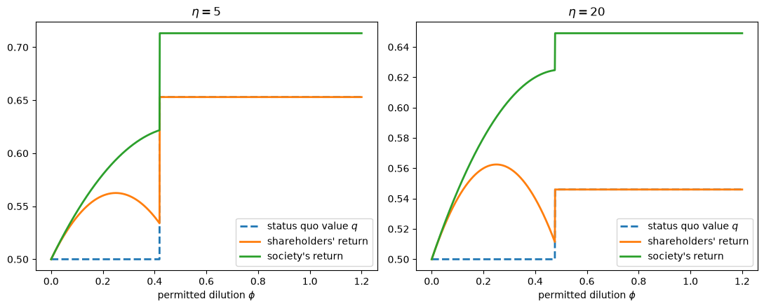
When \(\eta = 5\), departing from \(q^\ast\) is cheap for the manager, so the threat of a raid is a strong incentive, and shareholders are best off with any \(\phi\) large enough to make the manager respond to the threat, including unlimited dilution, case (1) of Proposition 3.
When \(\eta = 20\), departing from \(q^\ast\) is costly, so the manager stays near \(q^\ast\) anyway, and shareholders prefer to limit dilution to \(\phi = (1 - q^\ast)/2 = 0.25\), at which the manager ignores the threat of a raid and sets \(q = q^\ast\), while the tender price \(v - \phi\) stays high; this is case (2) of Proposition 3, in which \(\phi\) maximizes \((v - \phi) \Pr(\xi < \phi) + q^\ast \Pr(\xi \ge \phi)\).
In both cases society’s return is highest with unlimited dilution, as Proposition 5 of Grossman and Hart [1980] states, because society counts the raider’s profit along with the shareholders’ return; when \(\eta = 20\), the shareholders’ choice of \(\phi\) sacrifices managerial efficiency to get a higher tender price.
Exercise 56.3
Consider the takeover extension of Section 4.5 of Grossman and Hart [1982], with the technology, utility function, and normal distribution of the lecture and \(K = I^\ast = 1/4\).
Suppose, as in note 13 of Grossman and Hart [1982], that a raider can buy the firm for its market value \(V\) and, once in control, invests all of \(K\), so that the firm is worth \(g(K)/R\) to the raider, and that the raider’s cost \(\xi\) of a takeover is exponentially distributed with mean \(\mu_\xi\).
In the notation of the takeover section, the raider values the firm at \(v = g(K)/R\), its status quo value is \(q = V\), and buying the firm at \(V\) amounts to unlimited dilution.
Then a raid occurs when \(g(K)/R - V > \xi\), so that the probability that the firm is not taken over is
Show that, given \(I\), the debt that makes \(I\) the manager’s choice solves (56.5) with \(g(I)/R - I\) replaced by \(K - I\).
Treating \(I\) as the manager’s choice, compute the optimal investment, debt, probability of bankruptcy, probability of a takeover, and the manager’s expected utility for \(\mu_\xi \in \{0.02, 0.05, 0.1, 0.2, 1\}\).
Determine what the manager does when there is no threat of a takeover, \(\mu_\xi \to \infty\), and check your answer numerically.
Solution
Given \((V, D)\), the manager maximizes \(U(K - I) [1 - F(D - g(I))] \kappa(V)\), and since \(\kappa(V)\) does not depend on the manager’s choice of \(I\), the first-order condition is (56.3) with \(V - I\) replaced by \(K - I\).
So the debt that sustains \(I\) solves \(r(D - g(I)) = U'(K - I) / [U(K - I) \, g'(I)]\), and the manager’s expected utility along these equilibria is \(U(K - I) [1 - F(D(I) - g(I))] \kappa(g(I)/R)\).
def takeover_debt(I, K, firm):
    "The debt that makes I the manager's choice when capital K is fixed."
    y = U_prime(K - I, firm) / (U(K - I, firm) * g_prime(I, firm))
    return g(I, firm) + hazard_inverse(y, firm)

def no_takeover_prob(V, K, μ_ξ, firm):
    "Probability κ(V) that the firm is not taken over."
    return np.exp(-max(g(K, firm) / firm.R - V, 0) / μ_ξ)

def takeover_welfare(I, K, μ_ξ, firm):
    "The manager's expected utility at investment I under a takeover threat."
    D = takeover_debt(I, K, firm)
    return (U(K - I, firm) * (1 - F(D - g(I, firm), firm))
            * no_takeover_prob(g(I, firm) / firm.R, K, μ_ξ, firm))

K = I_star(firm)
print(f"upper bound U(K) = {U(K, firm):.4f}")
for μ_ξ in (0.02, 0.05, 0.1, 0.2, 1.0, np.inf):
    res = minimize_scalar(lambda I: -takeover_welfare(I, K, μ_ξ, firm),
                          bounds=(1e-8, K * (1 - 1e-8)), method='bounded',
                          options={'xatol': 1e-12})
    I = res.x
    D = takeover_debt(I, K, firm)
    V = g(I, firm) / firm.R
    print(f"μ_ξ = {μ_ξ:4}: I = {I:.4f}, D = {D:7.4f}, "
          f"P(bankruptcy) = {F(D - g(I, firm), firm):.3f}, "
          f"P(takeover) = {1 - no_takeover_prob(V, K, μ_ξ, firm):.3f}, "
          f"expected utility = {-res.fun:.4f}")
upper bound U(K) = 0.5000
μ_ξ = 0.02: I = 0.2080, D =  0.4983, P(bankruptcy) = 0.664, P(takeover) = 0.889, expected utility = 0.0077
μ_ξ = 0.05: I = 0.1876, D =  0.4164, P(bankruptcy) = 0.434, P(takeover) = 0.737, expected utility = 0.0372
μ_ξ =  0.1: I = 0.1638, D =  0.3468, P(bankruptcy) = 0.281, P(takeover) = 0.614, expected utility = 0.0814
μ_ξ =  0.2: I = 0.1290, D =  0.2615, P(bankruptcy) = 0.165, P(takeover) = 0.506, expected utility = 0.1437
μ_ξ =  1.0: I = 0.0258, D = -0.0262, P(bankruptcy) = 0.031, P(takeover) = 0.288, expected utility = 0.3269
μ_ξ =  inf: I = 0.0000, D = -0.4290, P(bankruptcy) = 0.000, P(takeover) = 0.000, expected utility = 0.5000
The smaller is \(\mu_\xi\), the stronger is the threat of a takeover, and the more the manager invests and borrows, accepting a higher probability of bankruptcy to hold down the probability of a takeover, which still rises as raids get cheaper.
The manager’s expected utility falls sharply as the threat grows.
Without a takeover threat, the manager’s expected utility is \(U(K - I) [1 - F(D(I) - g(I))]\), which the manager can push toward the upper bound \(U(K)\) by investing almost nothing and lending, so that \(D(I) \to -\infty\) and the probability of bankruptcy goes to zero.
The last row confirms this: with \(\mu_\xi = \infty\), the optimizer drives \(I\) to the lower end of its range, the manager lends, and expected utility approaches \(U(K) = 0.5\); the weakest finite threat in the table, \(\mu_\xi = 1\), already shows the manager lending, with \(D < 0\).
So, as Grossman and Hart argue, the threat of a takeover gives the manager a reason to issue debt, and the threat of bankruptcy is what makes the debt effective.
Exercise 56.4
Leland [1982] observed that if profit \(y = g(I) + s\) is publicly observed tomorrow, the manager could be disciplined without debt.
Suppose that the firm can commit to let the manager keep the perquisites with probability \(p(y)\), for any function \(p\) with values in \([0, 1]\); debt \(D\) corresponds to \(p(y) = 1\) for \(y \ge D\) and \(p(y) = 0\) otherwise.
Let \(\ell(s) = -f'(s)/f(s)\), which equals \(s/\sigma^2\) for our normal distribution, and let \(\psi(I)\) be the right side of (56.5).
Show that a rule \(p\) sustains the equilibrium with investment \(I\) and \(V = g(I)/R\) only if \(E[p(g(I) + s) \, \ell(s)] = \psi(I) \, E[p(g(I) + s)]\).
Show that \(E[\ell(s) \mid s \ge x] = r(x)\), so that for the threshold rule of debt this condition is (56.5).
Show that when \(\ell\) is increasing, the threshold rule maximizes the probability \(E[p(g(I) + s)]\) that the manager keeps the job among all rules that sustain \(I\).
Check this numerically by computing the manager’s highest expected utility under the logistic rules \(p(y) = 1/(1 + e^{-(y - m)/\tau})\) for several values of \(\tau\) and comparing it with the expected utility under debt.
Solution
Given \(V\), the manager maximizes \(U(V - I) \, P(I)\), where \(P(I) = E[p(g(I) + s)] = \int p(y) f(y - g(I)) \, dy\).
Since \(P'(I) = g'(I) \int p(y) [-f'(y - g(I))] \, dy = g'(I) \, E[p(g(I) + s) \, \ell(s)]\), the first-order condition \(U'/U = P'(I)/P(I)\) at \(V = g(I)/R\) is the stated condition.
For the threshold rule, \(E[\ell(s) \, \mathbb{1}\{s \ge x\}] = \int_x^\infty -f'(s) \, ds = f(x)\), so \(E[\ell(s) \mid s \ge x] = f(x)/[1 - F(x)] = r(x)\): the hazard rate is the average score of the states in which the manager keeps the job.
The condition in part 1 requires the \(p\)-weighted average score of the states in which the manager keeps the job to equal \(\psi(I) > 0\).
To keep as much probability as possible with a given average score, a rule should drop the states with the lowest scores, which, when \(\ell\) is increasing, are the states with the lowest profits.
Formally, maximizing \(\int p f\) subject to \(\int p \, (\ell - \psi) f = 0\) with a multiplier \(\mu\) sets \(p(s) = 1\) where \(1 + \mu [\ell(s) - \psi] > 0\), and \(\mu > 0\) because a lower tail of \(s\) has a negative average score, so the solution is an upper tail of \(s\), a threshold rule.
The next cell computes the manager’s best expected utility under logistic rules, which keep the job with a probability that rises smoothly with profit.
def logistic_rule(x, τ, firm, n=4001):
    "E p and E[p ℓ] for the rule p = expit((s - x) / τ), with s = y - g(I)."
    s = np.linspace(-8, 8, n) * firm.σ
    weights = norm.pdf(s / firm.σ) / firm.σ * (s[1] - s[0])
    p = expit((s - x) / τ) * weights
    return p.sum(), (p * s / firm.σ**2).sum()

def logistic_welfare(I, τ, firm):
    "Expected utility when a logistic rule with scale τ sustains I."
    c = g(I, firm) / firm.R - I
    ψ = U_prime(c, firm) / (U(c, firm) * g_prime(I, firm))

    def gap(x):
        P, P_ℓ = logistic_rule(x, τ, firm)
        return P_ℓ / P - ψ

    x = brentq(gap, -5 * firm.σ, 5 * firm.σ)
    return U(c, firm) * logistic_rule(x, τ, firm)[0]

for τ in (0.05, 0.02, 0.005):
    res = minimize_scalar(lambda I: -logistic_welfare(I, τ, firm),
                          bounds=(0.05, 0.3), method='bounded')
    print(f"logistic rule, τ = {τ:5}: I = {res.x:.4f}, "
          f"expected utility = {-res.fun:.4f}")
print(f"debt:                    I = {I_opt:.4f}, "
      f"expected utility = {manager_welfare(I_opt, firm):.4f}")
logistic rule, τ =  0.05: I = 0.1840, expected utility = 0.4324
logistic rule, τ =  0.02: I = 0.1964, expected utility = 0.4482
logistic rule, τ = 0.005: I = 0.1993, expected utility = 0.4515
debt:                    I = 0.1995, expected utility = 0.4517
Smoother rules leave the manager worse off, and they approach debt as \(\tau \to 0\).
So when profit is publicly observed and the manager can be punished only by dismissal, debt implements the best dismissal rule; as Leland noted, a promise to resign unless profit reaches \(D\) would do equally well, and in this model, where bankruptcy has no deadweight cost, the two give the same outcome.