76. Commitment and Flexibility in Policy#
76.1. Overview#
The lecture Temptation, Self-Control, and Consumption describes two reasons that a decision maker might care about the set of options from which it will later choose.
Kreps [1979] represents a decision maker who is uncertain about its future tastes and who therefore prefers a larger set of options to a smaller one.
Strotz [1956] and Gul and Pesendorfer [2001] describe decision makers who expect to be tempted and who can therefore prefer a smaller set.
This lecture studies designers who have both reasons at once and who choose a set of options from which somebody else will later choose.
The later chooser will know something that the designer does not, so the designer wants to leave it room to act on that knowledge.
The later chooser also ranks options differently than the designer does, in a direction that the designer knows, so the designer wants to remove some options.
We study three papers.
Amador et al. [2006] study a consumer who learns its taste for current consumption before it decides how much to save and who is tempted to consume too much.
The consumer’s earlier self chooses a subset of the budget set from which its later self will choose.
Amador, Werning, and Angeletos apply the same analysis to a society that writes a fiscal constitution for a government that knows the value of public spending and wants to spend too much.
Athey et al. [2005] study a monetary authority that has private information about the state of the economy and that is tempted to exploit a Phillips curve, as in Kydland and Prescott [1977] and Barro and Gordon [1983].
Society designs a dynamic mechanism that makes money growth depend on the history of the authority’s reports.
Dovis et al. [2026] study a society whose two factions disagree about policy and whose policymakers are biased relative to the factions that they represent.
They compare delegating policy to an executive agency that chooses from a mandate with delegating it to a legislature in which the two factions bargain.
In all three papers, under conditions on the distribution of shocks, the optimal set of options for a chooser who acts alone is an interval.
When the chooser is biased upward, the interval has a cap, and choosers whose shocks exceed a cutoff are bunched at the cap.
In the papers of Amador, Werning, and Angeletos and of Athey, Atkeson, and Kehoe, and in that of Dovis, Kirpalani, and Sublet when the two factions agree, the cap equals the action that the designer would choose for the bunched choosers if all that it knew about them was that their shocks exceed the cutoff.
Equivalently, at the cutoff, the chooser’s bias, measured in units of the shock, equals the expected amount by which the shock exceeds the cutoff, conditional on exceeding it.
For the consumer, the cap is a minimum level of savings; for the government, a ceiling on spending; for the monetary authority, a ceiling on inflation; for the executive agency, a mandate.
Athey, Atkeson, and Kehoe formulate their problem recursively, with continuation values as state variables, using the method of Abreu et al. [1990] that other lectures in this section also use.
Their main theorem states conditions under which the optimal mechanism holds continuation values constant, so that the dynamic mechanism reduces to a repeated static one.
Dovis, Kirpalani, and Sublet add political risk: policy varies with the identity of the faction in power, which society dislikes.
Political risk leads society to give an executive agency a narrower mandate.
It can also lead society to grant discretion to a legislature, in which policy departs from a default only when both factions agree, rather than to an executive agency.
Dovis, Kirpalani, and Sublet also ask whether a legislature that has given an agency a narrow mandate would later agree to relax it.
This lecture
describes how a designer ranks sets of options when another decision maker will choose from them,
solves a delegation problem with quadratic payoffs that has the structure common to the three papers,
describes the minimum-savings rules of Amador, Werning, and Angeletos and computes one,
describes the dynamic mechanism design problem of Athey, Atkeson, and Kehoe, computes their inflation cap, and compares it with reputation and with central bankers whose preferences differ from society’s, in the economy of the Phillips Curve Tradeoffs lectures of the intermediate series,
computes optimal mandates of Dovis, Kirpalani, and Sublet and compares executive delegation with legislative bargaining, and
describes three ways in which a mandate can matter, one of which is Gul and Pesendorfer’s.
We use the following imports.
import numpy as np
import matplotlib.pyplot as plt
from scipy.integrate import quad
from scipy.optimize import brentq, minimize, minimize_scalar
from scipy.stats import truncnorm
76.2. Flexibility and commitment#
Kreps [1979] studies a decision maker who chooses today a set of options from which it will choose one option later.
He asks why anyone would want flexibility and answers:
The individual choosing a menu would likely make some statement about being uncertain about something or other.
He calls this rationalization “uncertainty about future tastes.”
Kreps represents rankings of sets \(D\) in which a set is at least as good as each of its subsets, and that satisfy one further axiom, by
where the expectation is over a state \(s\) of the decision maker’s future tastes.
The lecture Temptation, Self-Control, and Consumption states his theorem.
Now suppose that the decision maker who chooses the set, whom we call the designer, differs from the decision maker who later chooses from it, whom we call the chooser.
The chooser observes \(s\) and picks
and the designer, whose utility is \(v(a, s)\), ranks sets by
Dekel and Lipman [2012] call a representation like (76.2) a random Strotz representation, because it evaluates a set by the choice that a randomly drawn chooser makes from it.
If \(u = v\), then (76.2) is Kreps’s representation (76.1) with \(U = v\).
A larger set is then never worse, and the designer gives the chooser every option.
If \(u\) differs from \(v\) in a direction that the designer knows, then the designer can strictly prefer a smaller set, as Strotz’s planner does.
The designer then trades off flexibility, which lets the chooser act on its information about \(s\), against commitment, which keeps the chooser from acting on its bias.
The designer can equivalently choose an allocation \(a(s)\) directly, subject to the incentive constraints
The set \(D\) is then the range of \(a(\cdot)\), and the incentive constraints say that each chooser picks \(a(s)\) from that range.
In all three papers, the designer cannot pay the chooser.
76.3. A delegation problem#
The following problem has the structure shared by the three papers.
The state \(s\) has a density \(f\) and a cumulative distribution function \(F\) on \([\underline s, \bar s]\).
The designer’s utility is \(v(a, s) = -\frac12 (a - s)^2\) and the chooser’s is \(u(a, s) = -\frac12 (a - s - b)^2\), with bias \(b > 0\).
In every state, the chooser wants an action that exceeds the designer’s preferred action by \(b\).
Raising a floor on actions would move the chooser’s choice upward in states in which it already exceeds the designer’s preferred action, so we consider sets of the form \(D = \{a : a \leq \bar a\}\).
The chooser picks \(\min(s + b, \bar a)\), so choosers with states \(s \geq s_h \equiv \bar a - b\) are bunched at the cap \(\bar a\).
The designer’s expected loss is
The loss is continuous at \(s_h\), so the terms that come from moving \(s_h\) cancel and
Setting \(L'(\bar a) = 0\) gives
or, equivalently,
Equation (76.3) says that the cap is the action that the designer would choose for the bunched choosers if all that it knew about them was that \(s \geq s_h\).
Equation (76.4) says that at the cutoff \(s_h\), the chooser’s bias equals the expected amount by which the state exceeds \(s_h\) among the bunched choosers.
Lowering the cap moves the bunched choosers whose states are below \(\bar a\) toward the designer’s preferred action and moves those whose states are above \(\bar a\) away from it.
For a log-concave density, the right side of (76.4) decreases with \(s_h\), so (76.4) has at most one solution.
If \(b = 0\), the designer gives the chooser full discretion, as in Kreps’s representation.
If \(b \geq E[s] - \underline s\), equation (76.4) has no solution, every chooser is bunched, and the designer sets \(\bar a = E[s]\), the best constant action; it gives the chooser no discretion.
When \(s\) is uniform on \([-1, 1]\), \(E[s - s_h \mid s \geq s_h] = (1 - s_h)/2\), so \(s_h = 1 - 2b\) and \(\bar a = 1 - b\) for \(b \leq 1\), and \(\bar a = 0\) for \(b \geq 1\).
For some densities, the designer can do better with a set that is not an interval.
Alonso and Matouschek [2008] and Amador and Bagwell [2013] give conditions under which the optimal set is an interval.
The distributional conditions in the three papers are conditions of this kind.
The following functions solve (76.4) for any density and for a bias that can depend on the cutoff, as it does in the consumer’s problem below.
def excess_mean(s_h, pdf, s_hi):
    "Return E[s - s_h | s ≥ s_h] for a density pdf on an interval with upper end s_hi."
    mass = quad(pdf, s_h, s_hi)[0]
    excess = quad(lambda s: (s - s_h) * pdf(s), s_h, s_hi)[0]
    return excess / mass


def cutoff(bias, pdf, s_lo, s_hi):
    """
    Return the cutoff s_h that solves bias(s_h) = E[s - s_h | s ≥ s_h].

    Return s_hi if the bias is not positive and s_lo if every chooser is bunched.
    """
    if bias(s_hi) <= 0:
        return s_hi
    gap = lambda s_h: excess_mean(s_h, pdf, s_hi) - bias(s_h)
    if gap(s_lo) <= 0:
        return s_lo
    return brentq(gap, s_lo, s_hi - 1e-9)


def optimal_cap(b, pdf, s_lo, s_hi):
    "Optimal cap for the chooser with constant bias b."
    s_h = cutoff(lambda s: b, pdf, s_lo, s_hi)
    if s_h == s_lo:                       # every chooser is bunched
        return quad(lambda s: s * pdf(s), s_lo, s_hi)[0]
    return s_h + b


def loss_with_cap(a_bar, b, pdf, s_lo, s_hi):
    "Designer's expected loss when the chooser picks min(s + b, a_bar)."
    s_h = min(max(a_bar - b, s_lo), s_hi)
    below = quad(lambda s: 0.5 * b**2 * pdf(s), s_lo, s_h)[0]
    above = quad(lambda s: 0.5 * (a_bar - s)**2 * pdf(s), s_h, s_hi)[0]
    return below + above
We check (76.4) against a direct minimization of the designer’s loss.
uniform_pdf = lambda s: 0.5               # density of s on [-1, 1]
σ_s = 0.5
normal_pdf = truncnorm(-1 / σ_s, 1 / σ_s, scale=σ_s).pdf

for name, pdf in (('uniform', uniform_pdf), ('truncated normal', normal_pdf)):
    for b in (0.2, 0.6):
        direct = minimize_scalar(lambda a: loss_with_cap(a, b, pdf, -1, 1),
                                 bounds=(-1, 1), method='bounded',
                                 options={'xatol': 1e-10}).x
        print(f"{name:>16}, b = {b}: cap from (cf-cutoff) = "
              f"{optimal_cap(b, pdf, -1, 1):.5f}, by minimization = {direct:.5f}")
         uniform, b = 0.2: cap from (cf-cutoff) = 0.80000, by minimization = 0.80000
         uniform, b = 0.6: cap from (cf-cutoff) = 0.40000, by minimization = 0.40000
truncated normal, b = 0.2: cap from (cf-cutoff) = 0.67345, by minimization = 0.67345
truncated normal, b = 0.6: cap from (cf-cutoff) = 0.12353, by minimization = 0.12353
The next figure plots the designer’s expected loss under full discretion, under the best constant action, and under the optimal cap, for a uniform state.
It also plots the optimal cap for both densities.
b_grid = np.linspace(0, 1.4, 57)
var_s = quad(lambda s: s**2 * uniform_pdf(s), -1, 1)[0]

loss_cap = [loss_with_cap(optimal_cap(b, uniform_pdf, -1, 1), b, uniform_pdf, -1, 1)
            for b in b_grid]

fig, axes = plt.subplots(1, 2, figsize=(11, 4))

ax = axes[0]
ax.plot(b_grid, b_grid**2 / 2, lw=2, label='full discretion')
ax.plot(b_grid, np.full_like(b_grid, var_s / 2), lw=2, label='best constant action')
ax.plot(b_grid, loss_cap, lw=2, label='optimal cap')
ax.set_xlabel('bias $b$')
ax.set_ylabel('expected loss')
ax.legend()

ax = axes[1]
for name, pdf in (('uniform', uniform_pdf), ('truncated normal', normal_pdf)):
    ax.plot(b_grid, [optimal_cap(b, pdf, -1, 1) for b in b_grid], lw=2,
            label=name)
ax.set_xlabel('bias $b$')
ax.set_ylabel(r'optimal cap $\bar a$')
ax.legend()

plt.tight_layout()
plt.show()
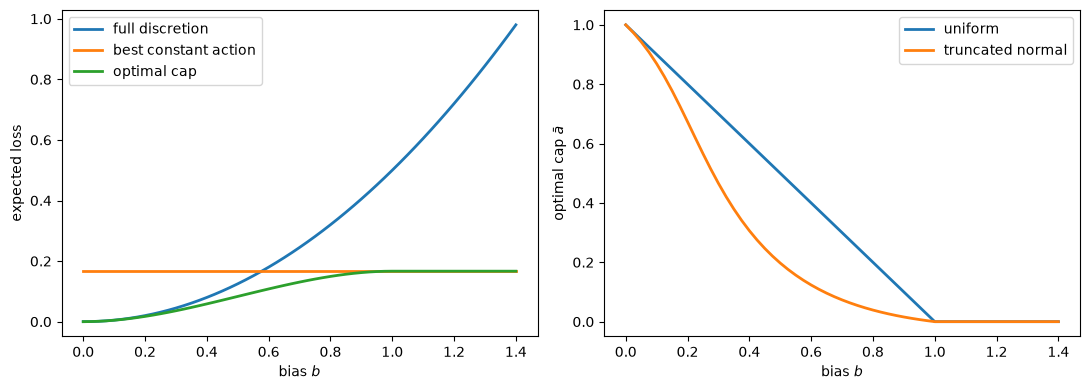
Fig. 76.1 Losses and caps under delegation#
The left panel shows the following:
For a small bias, the designer prefers full discretion to a constant action, and the optimal cap improves on full discretion only slightly.
For a large bias, the designer prefers a constant action to full discretion, and at \(b = 1\) the optimal cap becomes the constant action.
For intermediate biases, the optimal cap improves on both.
The right panel shows that the cap falls as the bias rises.
A truncated normal density puts less mass in the tails than the uniform density, so the expected excess over a cutoff is smaller, and the cap is lower for a given bias.
76.4. Commitment and flexibility for a consumer#
76.4.1. The consumer#
Amador et al. [2006] study a consumer who lives for two periods, consumes \(c\) in the first and \(k\) in the second, and faces the budget set
with the net interest rate normalized to zero.
At the start of the first period, the consumer learns a taste shock \(\theta\) that raises its marginal utility of current consumption.
The shock \(\theta\) has distribution \(F\) and density \(f\) on \(\Theta = [\underline \theta, \bar \theta]\), with \(E[\theta] = 1\).
Only the consumer observes \(\theta\).
Following Strotz [1956], Phelps and Pollak [1968], and Laibson [1997], Amador, Werning, and Angeletos model the consumer as two selves.
Self 1 chooses after it learns \(\theta\) and has utility
where \(U\) and \(W\) are increasing and concave and \(0 < \beta \leq 1\).
Self 0 chooses before \(\theta\) is drawn and has utility
They write: “We associate \(1 - \beta\) with the strength of temptation toward present consumption.”
Self 0 chooses a set \(C \subseteq B\), and self 1 then chooses from \(C\).
The authors state the trade-off:
Commitment is valued because it reduces temptation; flexibility is valued because it allows the use of valuable private information.
Choosing \(C\) is equivalent to choosing an allocation \(c(\theta), k(\theta)\) to maximize
subject to the incentive constraints
and the budget constraints \(c(\theta) + k(\theta) \leq y\).
The budget constraints allow self 0 to leave resources unspent, which amounts to “money burning.”
Two allocations serve as benchmarks.
The first-best allocation \((c^{fb}(\theta), k^{fb}(\theta))\) maximizes \(\theta U(c) + W(k)\) on \(B\); self 0 could achieve it if \(\theta\) were public and contractible.
The full-flexibility allocation \((c^f(\theta), k^f(\theta))\) maximizes \(\theta U(c) + \beta W(k)\) on \(B\); self 1 chooses it when \(C = B\).
76.4.2. Bunching at the top#
The indifference curves of \(\theta U + \beta W\) are the indifference curves of \((\theta / \beta) U + W\), so self 1 with shock \(\theta\) chooses as self 0 would choose for the shock \(\theta / \beta\).
Amador, Werning, and Angeletos explain why self 0 bunches the highest types (p. 374):
Informally, these types can make a case for their preferences. In contrast, self-1 types with \(\theta > \beta \bar \theta\) display a blatant desire for current consumption from self-0’s point of view. That is, there is no possible taste shock for self-0 that justifies self-1’s preferences.
Let
Their Proposition 2 states that an optimal allocation gives every type \(\theta \geq \theta_p\) the same bundle, a bundle on the budget line, where \(\theta_p\) is the lowest \(\hat \theta\) such that \(\int_{\theta'}^{\bar \theta} (1 - G(\theta)) \, d\theta \leq 0\) for all \(\theta' \geq \hat \theta\).
The integral equals
so an interior \(\theta_p\) solves
Equation (76.5) is an instance of (76.3).
When \(\theta_p\) is interior, the bunched bundle is the bundle that self 1 with shock \(\theta_p\) chooses from the budget line, which is the bundle that self 0 would choose for the shock \(\theta_p / \beta\).
Self 0’s expected utility from giving one bundle to every type above \(\theta_p\) is proportional to \(E[\theta \mid \theta \geq \theta_p] U(c) + W(k)\), so (76.5) says that the bunched bundle is the bundle that self 0 would choose for those types if all that it knew was that \(\theta \geq \theta_p\).
Self 1’s bias at the cutoff, measured in units of the shock, is \(\theta_p / \beta - \theta_p\), and (76.5) can be written as \(\theta_p / \beta - \theta_p = E[\theta - \theta_p \mid \theta \geq \theta_p]\), an instance of (76.4).
Equation (76.5) does not involve \(U\) or \(W\).
76.4.3. Minimum-savings rules#
Amador, Werning, and Angeletos then ask when bunching at the top is the only restriction that self 0 imposes.
They impose the following condition on the distribution of taste shocks.
Assumption A. For all \(\theta \leq \theta_p\), \(G(\theta)\) is nondecreasing.
When \(f\) is differentiable, Assumption A is equivalent to \(\theta f'(\theta) / f(\theta) \geq -(2 - \beta)/(1 - \beta)\) for \(\theta \leq \theta_p\).
Every nondecreasing density satisfies it, and so does every density with \(\theta f' / f\) bounded below when \(\beta\) is close enough to \(1\).
Their Propositions 3 and 4 state:
Theorem (Minimum-savings rules)
Suppose that \(\theta_p > \underline \theta\).
The allocation that gives each type \(\theta \leq \theta_p\) its full-flexibility bundle \((c^f(\theta), k^f(\theta))\) and each type \(\theta > \theta_p\) the bundle \((c^f(\theta_p), k^f(\theta_p))\) is optimal if Assumption A holds.
If Assumption A does not hold, no allocation of this form is optimal for any choice of \(\theta_p\).
Self 0 implements the optimal allocation by letting self 1 choose any bundle on the budget line that satisfies the minimum-savings rule \(k \geq k^f(\theta_p)\).
The consumer can impose the rule on itself by putting \(k^f(\theta_p)\) into an illiquid asset that pays the same return as a liquid asset but cannot be spent in the first period, a device studied by Laibson [1997].
If \(\theta_p = \underline \theta\), self 0 instead gives every type the best constant plan, the bundle on the budget line that maximizes \(E[\theta] U(c) + W(k)\), and the minimum-savings rule requires at least the savings in that bundle.
Exercise 1 works out an example.
Their Proposition 5 states that \(\theta_p\) increases with \(\beta\) and the minimum level of savings decreases with \(\beta\).
76.4.4. A computed rule#
With \(U = W = \log\) and \(y = 1\), the first-best and full-flexibility consumption rules are
For a uniform \(\theta\), \(G'(\theta) = (2 - \beta) f > 0\), so Assumption A holds, and (76.5) gives \(\theta_p = \beta \bar \theta / (2 - \beta)\) when this number exceeds \(\underline \theta\).
We set \(\theta \sim U[0.5, 1.5]\) and \(\beta = 0.7\) and compute \(\theta_p\) with the function cutoff, using the bias \((1 - \beta)\theta / \beta\).
θ_lo, θ_hi, β = 0.5, 1.5, 0.7
awa_pdf = lambda θ: 1 / (θ_hi - θ_lo)

θ_p = cutoff(lambda θ: (1 - β) * θ / β, awa_pdf, θ_lo, θ_hi)
print(f"θ_p from (cf-awa-cutoff): {θ_p:.5f}")
print(f"closed form β θ_hi / (2 - β): {β * θ_hi / (2 - β):.5f}")
print(f"β θ_hi: {β * θ_hi:.5f}")


def consumption(θ, weight):
    "Maximizer of θ log c + weight × log(1 - c)."
    return θ / (θ + weight)


def ex_ante_utility(c_rule):
    "Self 0's expected utility E[θ log c(θ) + log(1 - c(θ))]."
    g = lambda θ: (θ * np.log(c_rule(θ)) + np.log(1 - c_rule(θ))) * awa_pdf(θ)
    return quad(g, θ_lo, θ_hi, points=[θ_p])[0]


rules = {
    'first best': lambda θ: consumption(θ, 1),
    'minimum savings': lambda θ: consumption(min(θ, θ_p), β),
    'best constant': lambda θ: 0.5,
    'full flexibility': lambda θ: consumption(θ, β),
}
for name, rule in rules.items():
    print(f"{name:>17}: {ex_ante_utility(rule):.5f}")
θ_p from (cf-awa-cutoff): 0.80769
closed form β θ_hi / (2 - β): 0.80769
β θ_hi: 1.05000
       first best: -1.36447
  minimum savings: -1.37798
    best constant: -1.38629
 full flexibility: -1.39542
Among minimum-savings rules indexed by their cutoff, the cutoff \(\theta_p\) is best.
best_threshold = minimize_scalar(
    lambda t: -ex_ante_utility(lambda θ: consumption(min(θ, t), β)),
    bounds=(θ_lo, θ_hi), method='bounded', options={'xatol': 1e-10}).x
print(f"best cutoff by direct search: {best_threshold:.5f}")
best cutoff by direct search: 0.80769
The next figure plots the three consumption rules.
θ_grid = np.linspace(θ_lo, θ_hi, 201)

fig, ax = plt.subplots(figsize=(7, 4))
ax.plot(θ_grid, consumption(θ_grid, 1), lw=2, label='first best')
ax.plot(θ_grid, consumption(θ_grid, β), lw=2, label='full flexibility')
ax.plot(θ_grid, consumption(np.minimum(θ_grid, θ_p), β), lw=2,
        label='minimum savings')
ax.axvline(θ_p, color='k', ls=':', lw=1)
ax.set_xlabel(r'taste shock $\theta$')
ax.set_ylabel('first-period consumption $c$')
ax.legend()
plt.show()
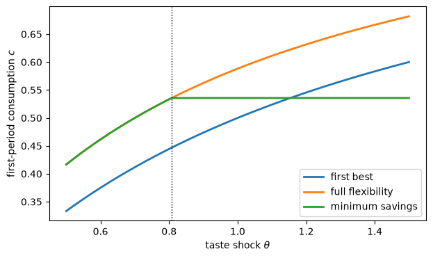
Fig. 76.2 First-period consumption under three rules#
The figure shows the following:
Self 1 consumes more than the first best for every \(\theta\) when it has full flexibility.
The minimum-savings rule leaves self 1’s choice unchanged for \(\theta < \theta_p\) and caps its consumption at \(c^f(\theta_p)\) above \(\theta_p\).
The cap binds for shocks well below \(\beta \bar \theta = 1.05\), the lowest shock for which self 1’s choice exceeds every choice that self 0 would want for some shock.
For these parameter values, self 0 prefers the best constant plan, \(c = 1/2\), to full flexibility, and it prefers the minimum-savings rule to both.
76.4.5. Self-control#
In their Section 4, Amador, Werning, and Angeletos give the consumer Gul–Pesendorfer preferences over sets:
which they adopt from Krusell et al. [2010].
In the notation of Temptation, Self-Control, and Consumption, the commitment utility is \(\theta U + W\), the temptation utility is \(\varphi (\theta U + \beta W)\), and \(\varphi > 0\) measures the cost of self-control.
As \(\varphi \to \infty\), these preferences converge to the two-selves model.
The consumer chooses from \(C\) the bundle that maximizes \((1 + \varphi)\theta U + (1 + \beta \varphi) W\), so it chooses as a self 1 with \(\beta\) replaced by \(\hat \beta = (1 + \beta \varphi)/(1 + \varphi)\), which lies between \(\beta\) and \(1\).
Options that the consumer does not choose lower \(P(C)\), because resisting them costs self-control.
The authors write that “commitment devices are valuable not only because they affect equilibrium behavior, but also because they may reduce the costs of exerting self-control.”
Their Propositions 6 and 7 extend the bunching and minimum-savings results under an analog of Assumption A.
Their Proposition 9 states that, when \(\beta\) and \(\varphi\) are known, the minimum level of savings decreases with \(\beta\) and increases with \(\varphi\).
76.4.6. Fiscal constitutions#
Amador, Werning, and Angeletos apply their results to a government that allocates resources between private consumption \(c\) and public services \(g\), with \(c + g \leq y\).
Citizens’ welfare is \(\theta U(g) + W(c)\), where \(\theta\) is the social value of public services.
The government maximizes \(\beta^{-1} \theta U(g) + W(c)\), where \(\beta^{-1} > 1\) measures its bias toward public spending.
Only the government observes \(\theta\).
A fiscal constitution is a subset of the budget set from which the government must choose.
The government’s indifference curves are those of self 1, so the analysis applies without change.
The authors write: “Proposition 2 shows that it is always optimal to limit government spending. Proposition 3 implies that, under Assumption A, only an upper cap on government spending is needed.”
76.5. Discretion in monetary policy#
76.5.1. The economy#
Athey et al. [2005] begin with a question that they attribute to Canzoneri:
The unsettled question in this debate is Canzoneri’s: What about when the monetary authority does have private information? What, then, is the optimal degree of monetary policy discretion?
In each period \(t = 0, 1, \ldots\), private agents first set the growth rates of their nominal wages; \(x_t\) denotes the average.
The monetary authority then observes a shock \(\theta_t\), drawn independently over time from a density \(p\) with distribution function \(P\) on \([\underline \theta, \bar \theta]\) and mean \(0\).
The monetary authority then chooses money growth \(\mu_t\), which equals inflation.
Unemployment is \(U + x_t - \mu_t\), where \(U > 0\) is the natural rate.
Social welfare in period \(t\) is
The monetary authority maximizes social welfare; only the authority observes \(\theta_t\), which affects the social cost of inflation.
The symbol \(U\) here denotes the natural rate of unemployment, not the utility function of the previous section.
Athey, Atkeson, and Kehoe denote the discount factor by \(\beta\); we denote it by \(\delta\) to avoid a clash with the previous section.
Three benchmarks come from (76.6).
The Ramsey policy \(\mu^R(\theta) = \theta/2\), with \(x = 0\), maximizes expected welfare when society can commit to a schedule and observes \(\theta\).
The expected Ramsey policy \(\mu^{ER} = 0\) is the best policy that does not depend on \(\theta\).
Given wages \(x\), the authority’s static best response is \(\mu^*(\theta; x) = (U + x + \theta)/2\); when wage setters expect it, \(x = U\) and \(\mu = U + \theta/2\).
They write: “Thus, for each type \(\theta\), the Nash policies are simply the Ramsey policies shifted up by \(U\).”
With the shock set to zero, (76.6) is the payoff in the one-period economy of The Credibility Problem, which follows chapter 3 of Sargent [1999] and Nancy Stokey’s version [Stokey, 1989] of the model of Kydland and Prescott [1977], with the slope of the Phillips curve set to one.
That lecture writes inflation as \(y\), expected inflation as \(x\), the natural rate as \(U^*\), and the slope of the Phillips curve as \(\theta\), so that its Phillips curve is \(U = U^* - \theta (y - x)\).
With slope one, its Nash and Ramsey inflation rates are \(U^*\) and \(0\), and its best response \(B(x) = (U^* + x)/2\) is the static best response \(\mu^*(0; x)\) here.
In this section, \(\theta\) is instead the authority’s private shock, and \(U\) is the natural rate.
The authority has both reasons to care about its set of options.
It knows \(\theta\), so society wants money growth to respond to \(\theta\), as in Kreps’s representation.
Given wages, it wants higher inflation than it would have chosen before wages were set, as in Kydland and Prescott [1977] and Barro and Gordon [1983].
Here the designer and the chooser have the same payoff function (76.6).
The chooser’s bias comes from the timing: wage setters act before the authority does.
The Ramsey policy is not incentive compatible when only the authority observes \(\theta\).
If society announced the schedule \(\mu^R\) and wage setters believed it, an authority with shock \(\theta\) would report \(\min\{U + \theta, \bar \theta\}\), the admissible report closest to \(U + \theta\), because \(\mu^R(U + \theta) = \mu^*(\theta; 0)\).
76.5.2. A recursive mechanism design problem#
Athey, Atkeson, and Kehoe study a direct revelation mechanism in which the monetary authority reports \(\theta_t\) each period and money growth depends on the history of reports.
Wage setters set \(x_t\) equal to expected money growth, given the history of reports.
Society maximizes \((1 - \delta) E \sum_{t=0}^\infty \delta^t R(x_t, \mu_t, \theta_t)\) subject to the constraint that the authority prefers to report truthfully after every history.
Following Abreu et al. [1990], they formulate the problem recursively.
Let \(\mathcal W\) be a compact set of candidate continuation values of social welfare, with largest element \(\bar w\).
Wages \(x\), a policy \(\mu(\cdot)\), and continuation values \(w(\cdot)\) are enforceable by \(\mathcal W\) if
An operator \(T\) maps \(\mathcal W\) into the set of values \(\int [(1 - \delta) R(x, \mu(\theta), \theta) + \delta w(\theta)] p(\theta) \, d\theta\) delivered by actions and continuation values that \(\mathcal W\) enforces.
The set of values of incentive-compatible mechanisms is the largest fixed point \(\mathcal W^* = T(\mathcal W^*)\).
The best value solves the best payoff problem
subject to enforceability by \(\mathcal W^*\).
Problem (76.7) has the structure of dynamic programming squared: the continuation values that the mechanism promises must themselves be values that the same problem can deliver.
Credible Government Policies applies the same operator to the repeated economy of The Credibility Problem, which has no private information, and computes the whole set of subgame perfect equilibrium values.
A mechanism is static if \(w(\theta) = \bar w\) for almost all \(\theta\).
They impose a single-crossing condition, \(R_{\mu \theta} > 0\), and a monotone hazard condition: \([1 - P(\theta)]R_{\theta \mu}/p(\theta)\) is strictly decreasing and \(P(\theta) R_{\theta \mu}/p(\theta)\) is strictly increasing.
For (76.6), \(R_{\theta\mu} = 1\), so the monotone hazard condition requires that \([1 - P(\theta)]/p(\theta)\) be strictly decreasing and \(P(\theta)/p(\theta)\) be strictly increasing.
Theorem (Static mechanism)
Under the single-crossing and monotone hazard conditions, the optimal mechanism is static.
In Optimal Unemployment Insurance and Repeated Moral Hazard, a planner rewards and punishes an agent by moving the agent’s promised value, and the planner’s own value moves in the opposite direction.
In the economy of Athey, Atkeson, and Kehoe, a lower continuation value punishes society along with the monetary authority.
They write:
The key feature of our problem that leads to the failure of the standard approach is that the continuation value enters positively into the payoff of both society and the monetary authority. Mathematically, these continuation values are analogous to the transfers between the principal and the agent in the standard principal-agent problem … In that problem, the transfers enter positively into the agent’s problem but negatively into the principal’s problem.
Their proof shows that whenever a mechanism uses variation in continuation values to make money growth rise with \(\theta\) over an interval, a variation that flattens money growth over that interval is feasible and raises welfare.
Credible Government Policies shows that, without private information, the best equilibrium is self-rewarding: it rewards adherence with the value that it promised, and it punishes only deviations, which the public sees and which never occur along the equilibrium path.
With private information, the public cannot see whether a report is true.
To make money growth rise with \(\theta\) without tempting the authority to misreport, a dynamic mechanism must lower continuation values after reports that truthful types make, so its punishments occur along the equilibrium path.
The theorem of Athey, Atkeson, and Kehoe states that, under the monotone hazard condition, the optimal mechanism imposes no such punishments.
In their Appendix B, they give examples in which the monotone hazard condition fails at a single point and the optimal mechanism is dynamic.
76.5.3. An inflation cap#
A policy has bounded discretion if, for some cutoff \(\theta^*\),
with \(x = \int \mu(\theta) p(\theta) \, d\theta\).
A policy has no discretion if it is constant, in which case it is best to set it equal to \(\mu^{ER}\).
Athey, Atkeson, and Kehoe show that the optimal policy has either bounded discretion or no discretion.
Society can implement it by legislating an inflation cap \(\bar \pi = \mu^*(\theta^*; x)\) and letting the authority and wage setters play the one-period equilibrium of the game with the cap in every period.
Types below \(\theta^*\) choose their static best responses, and types above \(\theta^*\) would like to choose higher inflation than \(\bar \pi\) and are stopped by the cap.
For the payoff (76.6), they show that the optimal policy
has complete discretion, \(\theta^* = \bar \theta\), if \(U = 0\),
has bounded discretion with a cutoff \(\theta^* < \bar \theta\) that decreases with \(U\) if \(0 < U < -\underline \theta\), and
is the expected Ramsey policy, with no discretion, if \(U \geq -\underline \theta\).
Their Appendix D characterizes the cutoff by
Since \(\int_{\theta^*}^{\bar \theta} (1 - P(\theta)) \, d\theta = (1 - P(\theta^*)) E[\theta - \theta^* \mid \theta \geq \theta^*]\), the second equation is
Equation (76.8) is an instance of (76.4).
The static best response of type \(\theta\) equals the Ramsey policy of type \(\theta + U + x\), so \(U + x\) is the authority’s bias measured in units of the shock.
The bias depends on expected inflation \(x\), which depends on the cutoff.
Substituting (76.8) into the cap gives
an instance of (76.3): the inflation cap is the expected Ramsey policy of the bunched types.
When \(\theta\) is uniform on \([-a, a]\) and \(0 \leq U \leq a\), (76.8) gives
Exercise 2 asks you to derive these formulas.
The following functions solve (76.8) for any density and compute expected welfare.
def aak_cutoff(U, pdf, θ_lo, θ_hi):
    """
    Return the cutoff θ* of the optimal bounded-discretion policy, or None
    if U ≥ -θ_lo, in which case the expected Ramsey policy is optimal.
    """
    if U <= 0:
        return θ_hi
    if U >= -θ_lo:
        return None

    def gap(t):
        x = U - quad(lambda θ: (θ - t) * pdf(θ), t, θ_hi)[0]
        return U + x - excess_mean(t, pdf, θ_hi)

    if gap(θ_lo + 1e-9) >= 0:            # U is within rounding error of -θ_lo
        return θ_lo
    return brentq(gap, θ_lo + 1e-9, θ_hi - 1e-9)


def aak_policy(U, θ_star, pdf, θ_hi):
    "Return the money growth rule and expected inflation x for a cutoff θ*."
    if θ_star is None:                   # expected Ramsey policy
        return (lambda θ: 0.0 * θ), 0.0
    x = U - quad(lambda θ: (θ - θ_star) * pdf(θ), θ_star, θ_hi)[0]
    return (lambda θ: (U + x + np.minimum(θ, θ_star)) / 2), x


def expected_welfare(μ, x, U, pdf, θ_lo, θ_hi):
    "Expected value of R(x, μ(θ), θ)."
    R = lambda θ: -0.5 * ((U + x - μ(θ))**2 + (μ(θ) - θ)**2)
    return quad(lambda θ: R(θ) * pdf(θ), θ_lo, θ_hi, limit=200)[0]
We take \(\theta\) uniform on \([-1, 1]\), compare the computed cutoffs with the closed form, and compare expected welfare under four policies.
a = 1.0
aak_pdf = lambda θ: 1 / (2 * a)

print("    U    θ* computed   θ* closed form   cap")
for U in (0.1, 0.3, 0.6, 0.9):
    θ_star = aak_cutoff(U, aak_pdf, -a, a)
    μ, x = aak_policy(U, θ_star, aak_pdf, a)
    print(f"  {U:.1f}     {θ_star: .5f}       {2 * a - np.sqrt(a**2 + 8 * a * U): .5f}"
          f"     {μ(a):.5f}")

print("\n    U    Ramsey    inflation cap   static Nash   expected Ramsey")
for U in (0.1, 0.3, 0.6, 0.9):
    θ_star = aak_cutoff(U, aak_pdf, -a, a)
    μ, x = aak_policy(U, θ_star, aak_pdf, a)
    values = [expected_welfare(lambda θ: θ / 2, 0.0, U, aak_pdf, -a, a),
              expected_welfare(μ, x, U, aak_pdf, -a, a),
              expected_welfare(lambda θ: U + θ / 2, U, U, aak_pdf, -a, a),
              expected_welfare(lambda θ: 0.0 * θ, 0.0, U, aak_pdf, -a, a)]
    print(f"  {U:.1f}  " + "    ".join(f"{v: .4f}   " for v in values))
    U    θ* computed   θ* closed form   cap
  0.1      0.65836        0.65836     0.41459
  0.3      0.15609        0.15609     0.28902
  0.6     -0.40832       -0.40832     0.14792
  0.9     -0.86356       -0.86356     0.03411

    U    Ramsey    inflation cap   static Nash   expected Ramsey
  0.1  -0.0883       -0.0923       -0.0933       -0.1717
  0.3  -0.1283       -0.1529       -0.1733       -0.2117
  0.6  -0.2633       -0.3237       -0.4433       -0.3467
  0.9  -0.4883       -0.5701       -0.8933       -0.5717
The Ramsey policy is not incentive compatible, so its welfare is an upper bound.
The inflation cap does better than both full discretion, the static Nash outcome, and no discretion, the expected Ramsey policy.
As \(U\) approaches \(-\underline \theta = 1\), the cap approaches \(0\) and the welfare of the capped policy approaches that of the expected Ramsey policy.
θ_grid = np.linspace(-a, a, 201)
U = 0.3
θ_star = aak_cutoff(U, aak_pdf, -a, a)
μ_cap, x_cap = aak_policy(U, θ_star, aak_pdf, a)

fig, axes = plt.subplots(1, 2, figsize=(11, 4))

ax = axes[0]
ax.plot(θ_grid, θ_grid / 2, lw=2, label='Ramsey')
ax.plot(θ_grid, U + θ_grid / 2, lw=2, label='static Nash')
ax.plot(θ_grid, np.zeros_like(θ_grid), lw=2, label='expected Ramsey')
ax.plot(θ_grid, μ_cap(θ_grid), lw=2, label='inflation cap')
ax.axvline(θ_star, color='k', ls=':', lw=1)
ax.set_xlabel(r'shock $\theta$')
ax.set_ylabel(r'money growth $\mu$')
ax.legend()

ax = axes[1]
U_grid = np.linspace(0, 1.2, 61)
θ_stars, caps = [], []
for U_val in U_grid:
    t = aak_cutoff(U_val, aak_pdf, -a, a)
    μ, _ = aak_policy(U_val, t, aak_pdf, a)
    θ_stars.append(-a if t is None else t)
    caps.append(μ(a))
ax.plot(U_grid, θ_stars, lw=2, label=r'cutoff $\theta^*$')
ax.plot(U_grid, caps, lw=2, label=r'inflation cap $\bar \pi$')
ax.set_xlabel('natural rate $U$')
ax.legend()

plt.tight_layout()
plt.show()
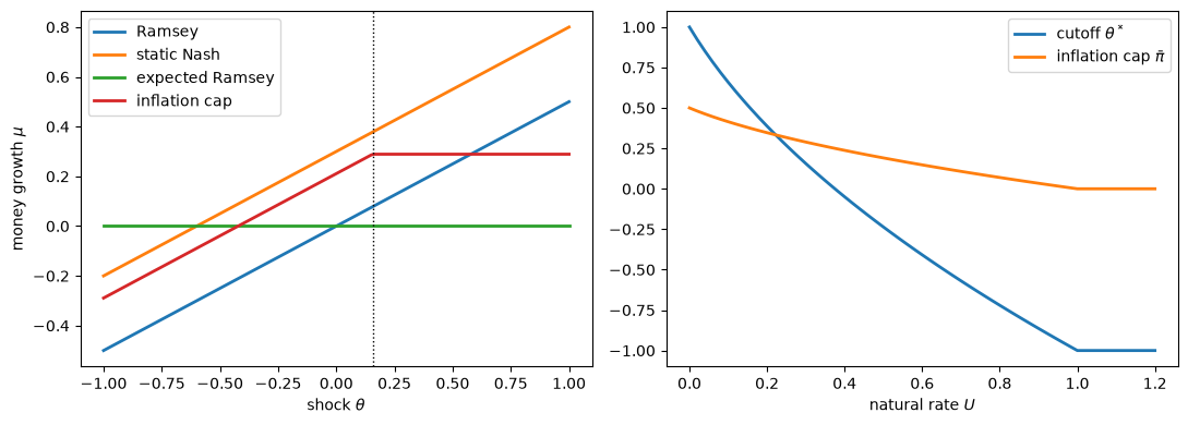
Fig. 76.3 Money growth policies and inflation caps#
The left panel, for \(U = 0.3\), shows that the capped policy coincides with the static best response for \(\theta < \theta^*\); there it lies above the Ramsey policy by \((U + x)/2\).
The right panel shows the cutoff and the cap falling as \(U\) rises and reaching \(-a\) and \(0\) at \(U = a\), where the expected Ramsey policy becomes optimal.
76.5.4. Reputation#
Athey, Atkeson, and Kehoe assume that society can legislate the inflation cap.
Without a legislated cap, the threat of returning forever to the static Nash outcome might deter the authority from exceeding \(\bar \pi\).
In Credible Government Policies, the same threat sustains the Ramsey outcome of the economy without private information when the discount factor satisfies \(\delta \geq 1/(2 + \theta^2)\), where \(\theta\) is the slope of the Phillips curve, so \(\delta \geq 1/3\) when the slope is one.
Wage setters see inflation above \(\bar \pi\), so it is a deviation that triggers the punishment.
Wage setters might not detect a deviation below \(\bar \pi\), but no type wants to deviate downward: types below \(\theta^*\) already choose their static best responses, and types above \(\theta^*\) want inflation higher than \(\bar \pi\).
Since \(R\) is quadratic in \(\mu\) with \(R_{\mu\mu} = -2\), a type \(\theta \geq \theta^*\) gains
in the period in which it deviates, and the type \(\bar \theta\) gains the most.
Let \(v^{cap}\) and \(v^N\) be expected one-period welfare under the capped policy and under static Nash.
Reverting to Nash after a deviation sustains the capped policy if \((1 - \delta)(\bar \theta - \theta^*)^2/4 \leq \delta (v^{cap} - v^N)\), that is, if
We compute \(\hat \delta\) for the optimal cap with \(\theta\) uniform on \([-1, 1]\).
print("    U      θ*      cap   v_cap - v_N   largest gain G   δ needed")
for U in (0.1, 0.3, 0.5, 0.7, 0.9):
    θ_star = aak_cutoff(U, aak_pdf, -a, a)
    μ, x = aak_policy(U, θ_star, aak_pdf, a)
    v_cap = expected_welfare(μ, x, U, aak_pdf, -a, a)
    v_N = expected_welfare(lambda θ: U + θ / 2, U, U, aak_pdf, -a, a)
    G = (a - θ_star)**2 / 4
    print(f"  {U:.1f}  {θ_star: .3f}   {μ(a):.3f}     {v_cap - v_N:.4f}"
          f"          {G:.4f}       {G / (G + v_cap - v_N):.3f}")
    U      θ*      cap   v_cap - v_N   largest gain G   δ needed
  0.1   0.658   0.415     0.0010          0.0292       0.965
  0.3   0.156   0.289     0.0204          0.1780       0.897
  0.5  -0.236   0.191     0.0758          0.3820       0.834
  0.7  -0.569   0.108     0.1752          0.6155       0.778
  0.9  -0.864   0.034     0.3233          0.8682       0.729
Nash reversion sustains the optimal cap only if \(\delta \geq \hat \delta\), and \(\hat \delta\) ranges from about \(0.73\) when \(U = 0.9\) to about \(0.97\) when \(U = 0.1\), far above the \(1/3\) that sustains the Ramsey outcome without private information.
The threshold is high for two reasons.
The types bunched at the cap are the ones most tempted to break it.
When \(U\) is small, the static Nash outcome is not much worse than the capped policy, so the threat of returning to it is weak.
Harsher punishments, such as the stick and carrot of Abreu [1988] that Credible Government Policies constructs, would lower these thresholds.
Exercise 5 finds the best capped policy that Nash reversion can sustain when the authority is less patient.
The calculation bears on the remark of Dovis, Kirpalani, and Sublet, described below, that reputation can keep a narrow mandate credible in a dynamic economy.
76.6. Legislatures and executive agencies#
76.6.1. The economy#
Dovis et al. [2026] study a static economy in which society chooses a policy \(\pi \in \mathbb{R}\) in response to a shock \(z \in [\underline z, \bar z]\) with distribution \(F\) and density \(f\).
The population consists of two factions, \(\theta \in \{\theta_L, \theta_H\}\), with population shares \(\alpha_L\) and \(\alpha_H\).
They call \(\Delta = \theta_H - \theta_L\) polarization.
A citizen of faction \(\theta\) has utility
and society’s welfare is \(v(\pi, z) = \sum_i \alpha_i w(\pi, z, \theta_i)\).
Each faction is represented by a policymaker with utility
where the bias \(\nu\) is common to both policymakers.
Faction \(i\) is in power with probability \(\alpha_i\).
The policymaker of faction \(\theta\) prefers \(\pi^f(z, \theta) = z + \theta + \nu\), while society prefers \(\pi^*(z) = z + \bar \theta\), with \(\bar \theta = \alpha_L \theta_L + \alpha_H \theta_H\).
The best constant policy is \(\bar \pi^* = E[z] + \bar \theta\); they note that Athey, Atkeson, and Kehoe call it the expected Ramsey policy.
Since \(u(\pi, z, \theta_H) = v(\pi, z) + (\nu + \alpha_L \Delta) \pi\) and \(u(\pi, z, \theta_L) = v(\pi, z) + (\nu - \alpha_H \Delta) \pi\), the two policymakers have different biases relative to society.
Dovis, Kirpalani, and Sublet call the bias small if \(\nu \in (-\alpha_L \Delta, \alpha_H \Delta)\), in which case society’s preferred policy lies between the two policymakers’ preferred policies.
When \(\nu = 0\) and \(\Delta = 0\), policymakers share society’s preferences, the value of a set \(D\) of policies is \(E \max_{\pi \in D} v(\pi, z)\), and (76.2) is Kreps’s representation (76.1).
Suppose next that \(\nu = 0\) and \(\Delta > 0\).
If society evaluated each state by the tastes of the faction in power, the value of \(D\) would be \(\sum_i \alpha_i E \max_{\pi \in D} w(\pi, z, \theta_i)\).
The faction in power would then be one more component of Kreps’s state, and a larger set would never be worse.
Dovis, Kirpalani, and Sublet instead evaluate every state with \(v\), so variation of policy with the faction in power lowers society’s welfare.
That variation is what they call political risk.
Society cannot write policy as a function of \(z\); it chooses only a set of policies and an institution.
They compare two institutions.
Under executive delegation, the policymaker of the faction in power chooses any policy in a set \(D\), its mandate.
Under legislative bargaining, the policymaker in power can choose a policy in \(D\) unilaterally, or any other policy if the policymaker of the other faction agrees.
76.6.2. Executive delegation#
Under executive delegation, the policymaker of faction \(\theta\) chooses \(\pi(z, \theta) \in \arg\max_{\pi \in D} u(\pi, z, \theta)\), and society chooses \(D\) to maximize \(\sum_i \alpha_i \int v(\pi(z, \theta_i), z) f(z) \, dz\).
Dovis, Kirpalani, and Sublet first restrict \(D\) to intervals \([\pi_l, \pi_h]\) and write \(\pi_h = \pi^f(z_h, \theta_L)\).
Define \(K(z) = \alpha_L F(z) + \alpha_H F(z - \Delta)\), the distribution function of \(z + \theta - \theta_L\), with density \(\kappa\); let \(E_\kappa\) denote an expectation under \(\kappa\); and let \(d(z) = F(z) - F(z - \Delta)\).
Their Lemma 1 states that if \(\Delta \alpha_L + \nu > 0\) and \(\alpha_H > 0\), the optimal cap binds, and an interior cap satisfies
When \(\Delta = 0\), \(K = F\) and (76.10) is (76.4) with \(b = \nu\).
The second term on the left is the cost of political risk.
They explain that “a looser cap not only increases flexibility, but also makes policy outcomes more sensitive to the identity of the policymaker.”
Their Proposition 1 states that the optimal set is an interval if and only if a distributional condition, their Assumption 1, holds; the uniform distribution satisfies it.
Their Lemma 2 states that, for a large enough bias or polarization, the optimal mandate is the single point \(\bar \pi^*\); they call this a narrow mandate.
76.6.3. Legislative bargaining#
Under legislative bargaining, let \(\pi_D(z, \theta)\) be the policy that faction \(\theta\)’s policymaker would choose from \(D\) on its own.
That policy is the outside option of the bargaining game.
The policymaker in power can implement any policy that the other faction’s policymaker, \(\hat \theta\), weakly prefers to the outside option, that is, any policy in
and it chooses its preferred policy in \(D \cup \mathcal R(z, \theta, D)\).
With quadratic utility, \(\mathcal R\) is the interval of policies no farther from \(\hat \theta\)’s preferred policy than the outside option is.
Their Proposition 2 states that if the bias is small, the optimal set \(D\) contains no intervals.
Removing an interval from \(D\) lowers the outside option of the faction in power and moves bargaining outcomes toward society’s preferred policy, and it costs no flexibility, because both factions can agree on any policy in the removed interval that both prefer.
They write: “Unlike in DE, drilling a hole in the delegation set does not create inefficiencies, because policymakers can renegotiate. In DE, such holes force bunching at inefficient policies; under LB, those inefficiencies are renegotiated away.”
Their Lemma 3 states that for large enough polarization, the optimal set is \(D = \{\bar \pi^*\}\), and factions never agree to depart from it.
76.6.4. Which institution is better?#
Their Proposition 3 states:
If \(\Delta > 0\) and the bias is small, society weakly prefers legislative bargaining to executive delegation.
If \(\nu > \text{sd}(z) + \alpha_H \Delta\) or \(\nu < -\text{sd}(z) - \alpha_L \Delta\), where \(\text{sd}(z)\) is the standard deviation of \(z\), society strictly prefers executive delegation.
If \(\Delta = 0\), society prefers executive delegation, strictly if \(\nu \neq 0\).
When the bias is small, bargaining between the factions gives policy room to respond to large shocks, and the outcome lies between the two factions’ preferred policies, near society’s.
When the bias is large, society wants to stop both factions from agreeing on a policy that suits their common bias, and a narrow mandate enforced by courts does that.
They conclude: “In this sense, Congress’s inaction can be a feature and not a problem.”
They also study a hybrid institution in which society restricts the set of policies on which the factions can agree; for a large bias, the best hybrid institution coincides with executive delegation.
76.6.5. Computations#
We take \(z\) uniform on \([-1, 1]\), \(\alpha_L = \alpha_H = 1/2\), \(\theta_L = -\Delta/2\), and \(\theta_H = \Delta/2\), so that \(\bar \theta = 0\), \(\pi^*(z) = z\), and \(\bar \pi^* = 0\).
Expectations over \(z\) are averages over the midpoints of a fine grid.
n_z = 2000
z_grid = -1 + (np.arange(n_z) + 0.5) * 2 / n_z
α_L = α_H = 0.5


def society_welfare(π_L, π_H):
    "Expected v(π, z) = zπ - π²/2 when faction L or faction H is in power."
    v = lambda π: np.mean(z_grid * π - π**2 / 2)
    return α_L * v(π_L) + α_H * v(π_H)


def de_policies(lo, hi, Δ, ν):
    "Policies that an executive of each faction chooses from the interval [lo, hi]."
    return [np.clip(z_grid + θ + ν, lo, hi) for θ in (-Δ / 2, Δ / 2)]


def best_de(Δ, ν):
    "Optimal interval mandate, found by searching over its endpoints."
    obj = lambda p: -society_welfare(*de_policies(p[0], p[0] + abs(p[1]), Δ, ν))
    results = [minimize(obj, p0, method='Nelder-Mead',
                        options={'xatol': 1e-9, 'fatol': 1e-13, 'maxiter': 5000})
               for p0 in ([-1.0, 2.0], [-0.5, 1.0], [-0.05, 0.1])]
    r = min(results, key=lambda r: r.fun)
    return r.x[0], r.x[0] + abs(r.x[1]), -r.fun


def lb_policies(D, Δ, ν):
    "Policies under legislative bargaining with the set of outside options D."
    D = np.atleast_1d(D)
    policies = []
    for θ, θ_other in ((-Δ / 2, Δ / 2), (Δ / 2, -Δ / 2)):
        p = z_grid + θ + ν                 # preferred policy of the faction in power
        q = z_grid + θ_other + ν           # preferred policy of the other faction
        π_D = D[np.argmin(np.abs(p[:, None] - D[None, :]), axis=1)]
        r = np.abs(π_D - q)                # the other faction accepts [q - r, q + r]
        policies.append(np.clip(p, q - r, q + r))
    return policies


def best_lb(Δ, ν, n_options=1, grid=np.linspace(-1.5, 1.5, 41)):
    "Best set of n_options outside options: a grid search, then a local search."
    obj = lambda D: -society_welfare(*lb_policies(D, Δ, ν))
    if n_options == 1:
        candidates = [[d] for d in grid]
    else:
        candidates = [[d1, d2] for i, d1 in enumerate(grid) for d2 in grid[i + 1:]]
    D_0 = min(candidates, key=obj)
    r = minimize(obj, D_0, method='Nelder-Mead',
                 options={'xatol': 1e-9, 'fatol': 1e-13})
    return np.sort(r.x), -r.fun
For a uniform \(z\), \(E[(z - c)^+]\) has a closed form, which gives the right side of (76.10).
We compare the cap from Lemma 1 with the cap found by searching over intervals.
def mean_excess_uniform(c):
    "E[max(z - c, 0)] for z uniform on [-1, 1]."
    return np.where(c < -1, -c, np.where(c > 1, 0.0, (1 - c)**2 / 4))


def lemma1_cap(Δ, ν):
    "Cap π_h = π^f(z_h, θ_L), with z_h from (cf-dks-cap), for z uniform on [-1, 1]."
    F = lambda z: np.clip((z + 1) / 2, 0, 1)
    K = lambda z: α_L * F(z) + α_H * F(z - Δ)
    d = lambda z: F(z) - F(z - Δ)

    def gap(z_h):
        tail = α_L * mean_excess_uniform(z_h) + α_H * mean_excess_uniform(z_h - Δ)
        return ν * (1 - K(z_h)) + Δ * α_L * α_H * d(z_h) - tail

    z_h = brentq(gap, -1 + 1e-9, 1 + Δ - 1e-9)
    return z_h - Δ / 2 + ν


for Δ, ν in ((0.0, 0.3), (1.0, 0.0), (1.0, 0.3), (1.0, 0.6)):
    lo, hi, _ = best_de(Δ, ν)
    print(f"Δ = {Δ}, ν = {ν}: cap from Lemma 1 = {lemma1_cap(Δ, ν):.4f}, "
          f"by search = {hi:.4f}")
Δ = 0.0, ν = 0.3: cap from Lemma 1 = 0.7000, by search = 0.7000
Δ = 1.0, ν = 0.0: cap from Lemma 1 = 0.5000, by search = 0.5000
Δ = 1.0, ν = 0.3: cap from Lemma 1 = 0.4169, by search = 0.4169
Δ = 1.0, ν = 0.6: cap from Lemma 1 = 0.2190, by search = 0.2190
When \(\Delta = 0\) and \(\nu = 0.3\), the cap is \(1 - \nu = 0.7\), as in the delegation problem.
With polarization \(\Delta = 1\) and no bias, political risk alone leads society to cap policy at \(0.5\).
The next figure plots policy as a function of the shock under the optimal executive mandate, in the left panel, and under legislative bargaining with the single outside option \(\bar \pi^* = 0\), in the right panel, for \(\nu = 0\) and \(\Delta = 1\).
Δ, ν = 1.0, 0.0
lo, hi, _ = best_de(Δ, ν)

fig, axes = plt.subplots(1, 2, figsize=(11, 4), sharey=True)
policies = (de_policies(lo, hi, Δ, ν), lb_policies([0.0], Δ, ν))
for ax, (π_L, π_H) in zip(axes, policies):
    ax.plot(z_grid, z_grid, 'k--', lw=1, label=r"society's preferred $\pi^*(z)$")
    ax.plot(z_grid, π_L, lw=2, label='faction $L$ in power')
    ax.plot(z_grid, π_H, lw=2, label='faction $H$ in power')
    ax.set_xlabel('shock $z$')
axes[0].set_ylabel(r'policy $\pi$')
axes[0].legend()
plt.tight_layout()
plt.show()
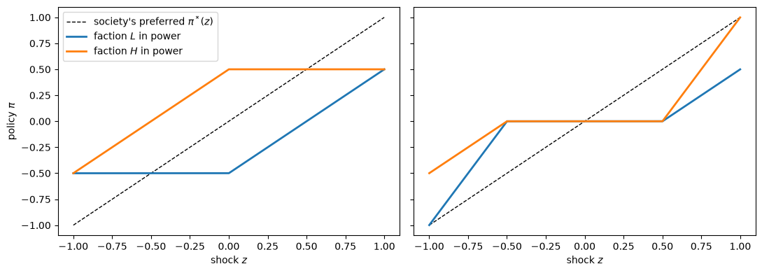
Fig. 76.4 Policies under delegation and bargaining#
The figure shows the following:
Under executive delegation, each faction’s policy responds one for one to \(z\) until it reaches the floor \(-0.5\) or the cap \(0.5\) of the mandate, and the two factions’ policies differ by \(1 - |z|\).
Under legislative bargaining, policy stays at \(0\) for \(z \in [-0.5, 0.5]\) and responds to larger shocks, because then the other faction agrees to a change.
Under legislative bargaining, the two factions’ policies coincide for \(|z| \leq 0.5\) and differ by at most \(0.5\) elsewhere.
The next figure plots society’s welfare against the bias for \(\Delta = 1\).
We compute the best legislative bargaining outcome with one and with two outside options; welfare under the optimal set of outside options is at least as high.
The dotted vertical lines mark \(\alpha_H \Delta\), the upper end of the small-bias region, and \(\text{sd}(z) + \alpha_H \Delta\), beyond which Proposition 3 says that executive delegation is strictly better.
Δ = 1.0
ν_grid = np.linspace(0, 1.5, 16)
W_de = [best_de(Δ, ν)[2] for ν in ν_grid]
W_lb1 = [best_lb(Δ, ν, 1)[1] for ν in ν_grid]
W_lb2 = [best_lb(Δ, ν, 2)[1] for ν in ν_grid]

fig, ax = plt.subplots(figsize=(8, 4.5))
ax.plot(ν_grid, W_de, 'o-', lw=2, label='executive delegation, optimal interval')
ax.plot(ν_grid, W_lb1, 's-', lw=2, label='legislative bargaining, one outside option')
ax.plot(ν_grid, W_lb2, '^-', lw=2, label='legislative bargaining, two outside options')
ax.axhline(society_welfare(z_grid, z_grid), color='k', ls='--', lw=1,
           label=r"society's preferred $\pi^*(z)$")
ax.axhline(0, color='k', lw=1, label=r'best constant policy $\bar \pi^*$')
ax.axvline(α_H * Δ, color='k', ls=':', lw=1)
ax.axvline(np.sqrt(1 / 3) + α_H * Δ, color='k', ls=':', lw=1)
ax.set_xlabel(r'bias $\nu$')
ax.set_ylabel('expected social welfare')
ax.set_ylim(-0.3, 0.2)
ax.legend(loc='lower left')
plt.show()
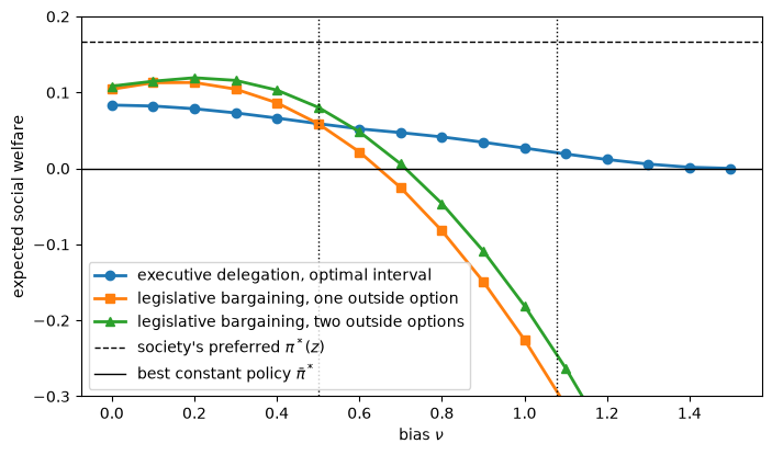
Fig. 76.5 Welfare under delegation and bargaining#
The figure shows the following:
For a small bias, legislative bargaining with one or two outside options yields higher welfare than the optimal executive mandate.
As the bias grows, welfare under legislative bargaining falls quickly, because the two factions agree on policies that suit their common bias.
For the largest biases, the optimal executive mandate is the narrow mandate \(\{0\}\), and welfare equals that of the best constant policy.
In this example, executive delegation yields higher welfare than legislative bargaining with one or two outside options for \(\nu \geq 0.6\), well below the bound \(\text{sd}(z) + \alpha_H \Delta \approx 1.08\) of Proposition 3.
Dovis, Kirpalani, and Sublet compute the threshold in the intermediate region numerically for a truncated normal shock.
76.6.6. Time inconsistency as the source of the bias#
Dovis, Kirpalani, and Sublet show that a bias like \(\nu\) arises from the time inconsistency studied by Athey, Atkeson, and Kehoe.
In their Section 7, the payoff of faction \(\theta\) is
where \(x\) is wage growth, \(\pi\) is money growth, and private agents set \(x\) equal to expected money growth before \(z\) is drawn and before the faction in power acts.
We take \(E[z] = 0\).
Society’s preferred allocation under commitment is \(\pi^*(z) = \bar \theta + z/2\), with \(x = \bar \theta\).
Without commitment, the policymaker of faction \(\theta\) chooses \(\pi^f(z, \theta; x) = (U + x + \theta + z)/2\), and the static equilibrium has \(x = U + \bar \theta\) and \(\pi(z, \theta) = \bar \theta + z/2 + U + (\theta - \bar \theta)/2\).
The static equilibrium differs from society’s preferred allocation by the inflation bias \(U\) and by the political risk \((\theta - \bar \theta)/2\).
With \(\lambda\) the Lagrange multiplier on the constraint that \(x\) equal expected money growth, they write that “it is as if society had biased preferences” \(R(x, \pi(z, \theta), z, \bar \theta) - \lambda \pi(z, \theta)\).
The bias \(\lambda\) now depends on the allocation and on the severity \(U\) of the time-inconsistency problem, as the bias \(U + x\) in (76.8) does.
Their Proposition 5 states that, for \(\Delta > 0\), there are thresholds \(U_L(\Delta)\) and \(U_H(\Delta)\) such that society weakly prefers legislative bargaining if \(U < U_L(\Delta)\) and strictly prefers executive delegation if \(U > U_H(\Delta)\).
76.6.7. Credibility#
A legislature that delegates policy to an agency can later change the agency’s mandate.
Dovis, Kirpalani, and Sublet call an institution and a set \(D\) credible if, for each faction in power, that faction’s policymaker prefers it to every alternative institution and set to which the other faction’s policymaker would agree.
Their Proposition 6 states that, with an exogenous bias that is not small, the optimal executive mandate is not credible.
They explain that “the gains from a binding mandate accrue only to society, which plays no role in the bargaining process,” so both factions agree to relax the mandate.
Their Proposition 7 states that, in the economy with time inconsistency, for \(U\) large enough, society prefers executive delegation and the optimal mandate is a credible narrow mandate at the best constant policy.
There, they write, “policymakers value the constraint themselves,” because a narrow mandate chosen before wages are set lowers expected inflation.
The mandate must be chosen before private agents set wages; once wages are set, every faction wants to best respond to them.
In a dynamic economy, they note, reputation can sustain the narrow mandate, as in Abreu [1988].
Their Proposition 8 states that, with an exogenous bias, legislative bargaining with a single outside option is always credible.
The lecture Accounting for Monetary and Fiscal Policy studies a government that delegates monetary policy to a central bank with an inflation target and can override the target when it needs revenue.
76.7. Three ways a mandate can matter#
The papers studied in this lecture and in Temptation, Self-Control, and Consumption describe three ways in which a set of options can matter to the decision maker who chooses it.
76.7.1. Through the choice made from it#
In representation (76.2), a set matters only through the choice that the chooser makes from it.
The bias \(\nu\) of Dovis, Kirpalani, and Sublet is an ingredient of this kind, as is the bias of self 1 in the two-selves model of Amador, Werning, and Angeletos.
76.7.2. Through options never chosen#
In Gul and Pesendorfer’s representation, options that the decision maker does not choose lower the value of a set, because they tempt it.
Fix \(z\), set \(\Delta = 0\), and treat the policymaker as a Gul–Pesendorfer decision maker whose commitment utility is society’s \(v(\cdot, z)\) and whose temptation utility is \(\nu \pi\), with \(\nu > 0\).
Its choice from \(D\) maximizes \(v + \nu \pi = u\), the same choice that the policymaker of Dovis, Kirpalani, and Sublet makes.
Its value of \(D\) is
society’s value less a cost of self-control that is proportional to the room above the chosen policy.
A Gul–Pesendorfer policymaker that ranks mandates before \(z\) is drawn by the expected value of this expression counts room above the chosen policy as a cost even in states in which the cap does not bind.
Exercise 3 shows that, for a uniform \(z\), such a policymaker sets a tighter cap than society does.
The self-control version of Amador, Werning, and Angeletos has the same structure.
Gul and Pesendorfer’s axiom of set betweenness rules out a strict preference for flexibility, so their representation, applied state by state, cannot by itself express the value of discretion; averaging over states, as in the preferences \(P(C)\) of Amador, Werning, and Angeletos, restores that value.
Dekel and Lipman [2012] study how far a ranking of sets can distinguish a Gul–Pesendorfer decision maker from a Strotz decision maker whose temptation is random.
76.7.3. Through other people’s expectations#
Kreps’s representation assumes that a set matters only through what is later chosen from it.
In the economies of Athey, Atkeson, and Kehoe and of Section 7 of Dovis, Kirpalani, and Sublet, wage setters see the inflation cap or mandate before they act, so the set also moves expected inflation.
Because wage setters respond to the mandate, each faction values a narrow mandate in Proposition 7 of Dovis, Kirpalani, and Sublet.
With an exogenous bias, a set affects nothing but the later choice, the factions gain nothing from a restriction that only society values, and the legislature relaxes the mandate, as Proposition 6 states.
76.8. Connections#
Kreps [1992] reads the 1979 representation as a model of contingencies that a decision maker cannot foresee, and he has institutions in mind (p. 259):
If one imagines that nonclassical contractual forms—relational contracting, for example—are adopted consciously by the transacting parties because those parties wish to provide themselves with governance provisions by which the unforeseen can be met, then it seems patent that those individuals are acting in anticipation of unforeseen contingencies.
A legislature whose factions can agree after a shock is such a provision.
Society in the model of Dovis, Kirpalani, and Sublet cannot write a mandate as a function of \(z\), so \(z\) is uncontractable, and Temptation, Self-Control, and Consumption quotes Kreps’s statement that at the level of static choice unforeseen and uncontractable contingencies are observationally equivalent.
The trade-off between Strotz’s case for a smaller set and Kreps’s case for a larger one is old.
On 16 August 1787, the Constitutional Convention debated whether to forbid the federal government to issue paper money (Sargent [2008], p. 7, n. 3).
Gouverneur Morris, Oliver Ellsworth, and James Madison recognized a time-inconsistency problem and made Strotz’s case.
Edmund Randolph and George Mason doubted the wisdom of tying the government’s hands, on the ground that no one can foresee all contingencies, and made Kreps’s case.
Kreps [1979] (pp. 567–568) offers advice that applies to anyone who proposes to widen or narrow a mandate:
If an individual expressed a desire for flexibility and approached me for advice, I would advise him (i) to try to assess what is the uncertainty that he perceives and (ii) to consider, if only to sharpen his assessments, how he would rank “opportunity sets contingent on the states” that he perceives.
Addressed to a designer of a mandate, the advice asks it to name the states in which room added to or removed from the mandate would be used and whose tastes would choose there.
The Rise and Fall of U.S. Inflation describes two accounts in Sargent [1999] of the rise and fall of U.S. inflation, the triumph of natural-rate theory and the vindication of econometric policy evaluation.
Sargent ends the book with a hope:
In the end, though our simulations and econometric evidence bolster the vindication of econometric policy evaluation story, we hope that this is the wrong story. We hope instead that policy makers somehow have learned a correct rational expectations version of the natural rate hypothesis and to commit themselves to low inflation.
The Rise and Fall of U.S. Inflation adds that theoretical work after Kydland and Prescott [1977], such as Rogoff [1985], “insists that durable low inflation must rest on commitment mechanisms that keep a monetary authority from choosing sequentially.”
The papers studied in this lecture describe commitment mechanisms of that kind and the conditions under which a legislature keeps them.
Athey, Atkeson, and Kehoe write that, in an economy with a publicly observed state, “society would specify a rule for setting the inflation cap with public information. We interpret such a rule as a type of inflation targeting.”
Dovis, Kirpalani, and Sublet find that a legislature keeps a narrow mandate when the bias that the mandate restrains comes from time inconsistency, as in the Phillips-curve economy of their Section 7, and relaxes the mandate when the bias is exogenous.
Other lectures connect to this one:
The Credibility Problem and Credible Government Policies study one-period and repeated versions of the economy of Athey, Atkeson, and Kehoe without private information.
The Rise and Fall of U.S. Inflation and the lectures that follow it study a government that learns about the Phillips curve as it sets inflation.
Time Inconsistency of Ramsey Plans and Sustainable Plans for a Calvo Model study time inconsistency of Ramsey plans and sustainable plans in a model of inflation.
Competitive Equilibria of a Model of Chang and Credible Government Policies in a Model of Chang apply the method of Abreu et al. [1990] that Athey, Atkeson, and Kehoe use.
Optimal Unemployment Insurance and Repeated Moral Hazard study mechanisms whose promised values move over time.
Accounting for Monetary and Fiscal Policy studies a central bank whose inflation target a government can override.
76.9. Exercises#
Exercise 76.1
Take the consumer of Amador, Werning, and Angeletos with \(U = W = \log\), \(y = 1\), and \(\theta\) uniform on \([\underline \theta, \bar \theta] = [0.5, 1.5]\).
Show that \(\theta_p = \max\{\underline \theta, \beta \bar \theta / (2 - \beta)\}\).
Show that when \(\theta_p > \underline \theta\) the minimum level of savings is \(k_{\min} = \beta/(\theta_p + \beta)\), and find the optimal plan when \(\theta_p = \underline \theta\).
Plot \(\theta_p\) and \(k_{\min}\) against \(\beta \in (0, 1]\), and check Proposition 5 of Amador, Werning, and Angeletos.
For several values of \(\beta\), compare \(\theta_p\) with the cutoff that a direct search over minimum-savings rules finds.
Solution
For a uniform \(\theta\), \(E[\theta \mid \theta \geq \theta_p] = (\theta_p + \bar \theta)/2\), so (76.5) is \(\theta_p / \beta = (\theta_p + \bar \theta)/2\), with solution \(\theta_p = \beta \bar \theta / (2 - \beta)\).
This solution lies above \(\underline \theta = 0.5\) if and only if \(1.5 \beta > 0.5 (2 - \beta)\), that is, if and only if \(\beta > 1/2\).
When \(\theta_p > \underline \theta\), the bunched bundle is self 1’s choice at \(\theta_p\), so \(c = \theta_p / (\theta_p + \beta)\) and \(k_{\min} = 1 - c = \beta / (\theta_p + \beta)\).
When \(\beta \leq 1/2\), every type is bunched, and self 0 gives all types the bundle that maximizes \(E[\theta] \log c + \log(1 - c)\), namely \(c = k = 1/2\).
Every type then wants to consume at least \(1/2\), because \(c^f(\underline \theta) = 0.5/(0.5 + \beta) \geq 1/2\), so the minimum-savings rule \(k \geq 1/2\) implements this rigid plan.
At \(\beta = 1/2\) both formulas give \(k_{\min} = 1/2\).
def awa_rule(β, θ_lo=0.5, θ_hi=1.5):
    "Return the cutoff θ_p and the minimum level of savings."
    θ_p = max(θ_lo, β * θ_hi / (2 - β))
    k_min = β / (θ_p + β) if θ_p > θ_lo else 0.5
    return θ_p, k_min


β_grid = np.linspace(0.05, 1, 96)
θ_ps, k_mins = zip(*[awa_rule(b) for b in β_grid])

fig, ax = plt.subplots(figsize=(7, 4))
ax.plot(β_grid, θ_ps, lw=2, label=r'cutoff $\theta_p$')
ax.plot(β_grid, k_mins, lw=2, label=r'minimum savings $k_{\min}$')
ax.set_xlabel(r'$\beta$')
ax.legend()
plt.show()
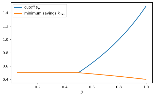
The cutoff rises and the minimum level of savings falls as \(\beta\) rises, as Proposition 5 states.
At \(\beta = 1\), \(\theta_p = \bar \theta\) and \(k_{\min} = 0.4 = k^f(\bar \theta)\), so the rule does not bind: with no temptation, self 0 gives self 1 full flexibility.
def utility_of_cutoff(t, β, θ_lo=0.5, θ_hi=1.5):
    "Self 0's expected utility from the minimum-savings rule with cutoff t."
    c = lambda θ: min(θ, t) / (min(θ, t) + β)
    g = lambda θ: θ * np.log(c(θ)) + np.log(1 - c(θ))
    return quad(g, θ_lo, θ_hi, points=[t])[0] / (θ_hi - θ_lo)


for b in (0.6, 0.7, 0.8, 0.9):
    search = minimize_scalar(lambda t: -utility_of_cutoff(t, b), bounds=(0.5, 1.5),
                             method='bounded', options={'xatol': 1e-10}).x
    print(f"β = {b}: θ_p = {awa_rule(b)[0]:.5f}, direct search = {search:.5f}")
β = 0.6: θ_p = 0.64286, direct search = 0.64286
β = 0.7: θ_p = 0.80769, direct search = 0.80769
β = 0.8: θ_p = 1.00000, direct search = 1.00000
β = 0.9: θ_p = 1.22727, direct search = 1.22727
Exercise 76.2
Take the economy of Athey, Atkeson, and Kehoe with \(\theta\) uniform on \([-a, a]\).
Use (76.8) and the equation for \(x\) to show that \(\theta^* = 2a - \sqrt{a^2 + 8aU}\) and \(\bar \pi = (a + \theta^*)/4\) for \(0 \leq U \leq a\).
Check that \(\theta^* = a\) when \(U = 0\) and \(\theta^* = -a\) when \(U = a\), as the result of Athey, Atkeson, and Kehoe requires.
Replace the uniform density by a normal density with mean \(0\) and standard deviation \(0.4\), truncated to \([-1, 1]\), and plot the cutoff and the cap against \(U\) for both densities.
Solution
For a uniform \(\theta\) on \([-a, a]\) and \(m = a - \theta^*\), \(\int_{\theta^*}^{a} (\theta - \theta^*) p(\theta) \, d\theta = m^2/(4a)\) and \(E[\theta - \theta^* \mid \theta \geq \theta^*] = m/2\).
The equation for \(x\) gives \(x = U - m^2/(4a)\), and (76.8) gives \(U + x = m/2\).
Eliminating \(x\) gives \(m^2 + 2am - 8aU = 0\), whose positive root is \(m = -a + \sqrt{a^2 + 8aU}\), so \(\theta^* = a - m = 2a - \sqrt{a^2 + 8aU}\).
The cap is \(\bar \pi = (U + x + \theta^*)/2 = (m/2 + \theta^*)/2 = (a + \theta^*)/4\).
At \(U = 0\), \(\theta^* = 2a - a = a\), and at \(U = a\), \(\theta^* = 2a - 3a = -a\).
σ_θ = 0.4
normal_θ_pdf = truncnorm(-1 / σ_θ, 1 / σ_θ, scale=σ_θ).pdf
U_grid = np.linspace(0, 1.2, 49)

fig, axes = plt.subplots(1, 2, figsize=(11, 4))
for name, pdf in (('uniform', aak_pdf), ('truncated normal', normal_θ_pdf)):
    θ_stars, caps = [], []
    for U_val in U_grid:
        t = aak_cutoff(U_val, pdf, -1, 1)
        μ, _ = aak_policy(U_val, t, pdf, 1)
        θ_stars.append(-1 if t is None else t)
        caps.append(μ(1.0))
    axes[0].plot(U_grid, θ_stars, lw=2, label=name)
    axes[1].plot(U_grid, caps, lw=2, label=name)
axes[0].plot(U_grid, np.maximum(2 - np.sqrt(1 + 8 * U_grid), -1), 'k:',
             lw=2, label='closed form, uniform')
axes[0].set_ylabel(r'cutoff $\theta^*$')
axes[1].set_ylabel(r'inflation cap $\bar \pi$')
for ax in axes:
    ax.set_xlabel('natural rate $U$')
    ax.legend()
plt.tight_layout()
plt.show()
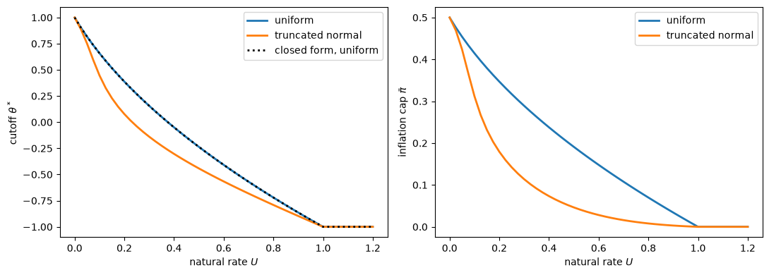
The truncated normal density has the same support as the uniform density, so in both cases no discretion becomes optimal at \(U = -\underline \theta = 1\).
The truncated normal puts less mass near the ends of the support, so the expected excess over a cutoff is smaller, and for a given \(U\) the cutoff and the cap are lower.
Exercise 76.3
Take the economy of Dovis, Kirpalani, and Sublet with \(\Delta = 0\), \(\bar \theta = 0\), \(\nu \in (0, 1)\), and \(z\) uniform on \([-1, 1]\), and consider mandates \(D = \{\pi : \pi \leq c\}\).
Show that society’s optimal cap is \(c = 1 - \nu\).
A Gul–Pesendorfer policymaker with commitment utility \(v(\pi, z) = z\pi - \pi^2/2\) and temptation utility \(\nu \pi\) ranks mandates by \(E\big[v(\pi_D(z), z) - \nu(c - \pi_D(z))\big]\). Show that its optimal cap is \(c = (1 - \sqrt{\nu})^2\).
Show that \((1 - \sqrt{\nu})^2 < 1 - \nu\), and verify both caps numerically.
Explain why the Gul–Pesendorfer policymaker chooses the tighter cap.
Solution
The policymaker chooses \(\pi_D(z) = \min(z + \nu, c)\), so the cap binds when \(z > c - \nu\).
Society’s expected welfare has derivative
which is zero at \(c = 1 - \nu\).
The Gul–Pesendorfer value equals \(E[v(\pi_D(z), z) + \nu \pi_D(z)] - \nu c\), and \(v + \nu \pi = u\) has derivative \(z + \nu - \pi\) with respect to \(\pi\), so
which is zero at \(1 + \nu - c = 2 \sqrt{\nu}\), that is, at \(c = (1 - \sqrt{\nu})^2\).
Since \((1 - \sqrt{\nu})^2 = 1 - \nu - 2\sqrt{\nu}(1 - \sqrt{\nu})\), the Gul–Pesendorfer cap is lower for \(\nu \in (0, 1)\).
z_fine = -1 + (np.arange(20000) + 0.5) / 10000

def society_value(c, ν):
    π = np.minimum(z_fine + ν, c)
    return np.mean(z_fine * π - π**2 / 2)

def gp_value(c, ν):
    π = np.minimum(z_fine + ν, c)
    return np.mean(z_fine * π - π**2 / 2 - ν * (c - π))

for ν in (0.1, 0.25, 0.5, 0.75):
    c_soc = minimize_scalar(lambda c: -society_value(c, ν), bounds=(-1, 2),
                            method='bounded', options={'xatol': 1e-10}).x
    c_gp = minimize_scalar(lambda c: -gp_value(c, ν), bounds=(-1, 2),
                           method='bounded', options={'xatol': 1e-10}).x
    print(f"ν = {ν}: society {c_soc:.4f} (1 - ν = {1 - ν:.4f}), "
          f"Gul–Pesendorfer {c_gp:.4f} ((1 - √ν)² = {(1 - np.sqrt(ν))**2:.4f})")
ν = 0.1: society 0.9000 (1 - ν = 0.9000), Gul–Pesendorfer 0.4675 ((1 - √ν)² = 0.4675)
ν = 0.25: society 0.7500 (1 - ν = 0.7500), Gul–Pesendorfer 0.2500 ((1 - √ν)² = 0.2500)
ν = 0.5: society 0.5000 (1 - ν = 0.5000), Gul–Pesendorfer 0.0858 ((1 - √ν)² = 0.0858)
ν = 0.75: society 0.2500 (1 - ν = 0.2500), Gul–Pesendorfer 0.0179 ((1 - √ν)² = 0.0179)
For a given cap \(c\), the Gul–Pesendorfer policymaker chooses \(\min(z + \nu, c)\) in every state, as the policymaker of Dovis, Kirpalani, and Sublet does, so the two optimal caps differ only because society and the Gul–Pesendorfer policymaker value a cap differently.
In states in which the cap does not bind, raising the cap leaves society’s welfare unchanged but raises the Gul–Pesendorfer policymaker’s cost of self-control, \(\nu(c - \pi_D(z))\), because it adds tempting options that the policymaker must resist.
The Gul–Pesendorfer policymaker therefore gains from a lower cap even in states in which the cap does not bind.
Exercise 76.4
Take the economy with a Phillips-curve shock \(\zeta\) that the authority sees and the public does not, with \(U^* = 5\) and \(\zeta\) uniform on \([-\sqrt{3}\sigma_\zeta, \sqrt{3}\sigma_\zeta]\).
Plot society’s expected loss, net of \(U^{*2}/2\), under the optimal inflation cap, the best Rogoff banker, and Blinder’s authority, against \(\sigma_\zeta \in [0.5, 8]\). Use the formula \(\frac12 \big[(U^*/\alpha)^2 + \sigma_\zeta^2 (\alpha^2 + 1)/(1 + \alpha)^2\big]\) for the loss under a Rogoff banker with weight \(\alpha\) and \(\sigma_\zeta^2/4\) for the loss under Blinder’s authority.
Suppose that society appoints a Rogoff banker with weight \(\alpha\) and also legislates a cap \(c\), so that inflation is \(y = \min\{(U^* + \zeta + x)/(1 + \alpha), c\}\), with \(x = E y\). For \(\sigma_\zeta \in \{1, 2.5, 5\}\), find the pair \((\alpha, c)\) that minimizes society’s expected loss. Does the cap bind?
Explain the answer to part 2.
Solution
The loss under a Rogoff banker comes from substituting \(x = U^*/\alpha\) and \(y = U^*/\alpha + \zeta/(1 + \alpha)\) into \(U = U^* + \zeta + x - y\).
For the cap, we use the functions aak_cutoff and aak_policy with \(U^*\) in place of \(U\) and \(\zeta\) in place of \(\theta\).
U_star = 5.0
σ_grid = np.linspace(0.5, 8, 31)

def rogoff_loss(α, σ_ζ):
    return 0.5 * ((U_star / α)**2 + σ_ζ**2 * (α**2 + 1) / (1 + α)**2)

loss_cap, loss_rogoff = [], []
for σ_ζ in σ_grid:
    a_ζ = np.sqrt(3) * σ_ζ
    pdf_ζ = lambda ζ: 1 / (2 * a_ζ)
    μ, x = aak_policy(U_star, aak_cutoff(U_star, pdf_ζ, -a_ζ, a_ζ), pdf_ζ, a_ζ)
    loss_cap.append(-expected_welfare(μ, x, U_star, pdf_ζ, -a_ζ, a_ζ) - U_star**2 / 2)
    loss_rogoff.append(minimize_scalar(lambda α: rogoff_loss(α, σ_ζ),
                                       bounds=(1, 1000), method='bounded').fun)

fig, ax = plt.subplots(figsize=(7, 4))
ax.plot(σ_grid, loss_cap, lw=2, label='optimal inflation cap')
ax.plot(σ_grid, loss_rogoff, lw=2, label='best Rogoff banker')
ax.plot(σ_grid, σ_grid**2 / 4, lw=2, label="Blinder's authority")
ax.axvline(U_star / np.sqrt(3), color='k', ls=':', lw=1)
ax.set_xlabel(r'$\sigma_\zeta$')
ax.set_ylabel(r'expected loss minus $U^{*2}/2$')
ax.legend()
plt.show()
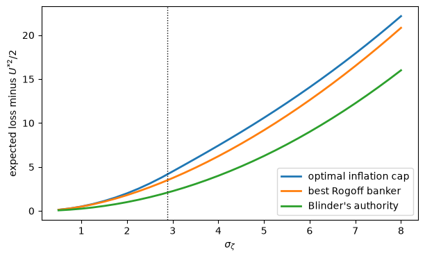
Blinder’s authority has the lowest loss for every \(\sigma_\zeta\), and the best Rogoff banker has a lower loss than the optimal cap for every \(\sigma_\zeta\).
To the left of the dotted line, \(U^* \geq \sqrt{3}\sigma_\zeta\), the optimal cap is \(0\), and its loss is \(\sigma_\zeta^2/2\), the loss of the expected Ramsey policy.
For part 2, we compute expected values on a fine grid of shocks, solve for \(x\) given \((\alpha, c)\), search over a grid of pairs, and refine the best pair.
ζ_nodes = -1 + (np.arange(4000) + 0.5) / 2000      # midpoints of a grid on [-1, 1]

def banker_with_cap(α, c, a_ζ):
    "Society's expected loss, net of U*²/2, with a Rogoff banker α and a cap c."
    ζ = a_ζ * ζ_nodes
    choice = lambda x: np.minimum((U_star + ζ + x) / (1 + α), c)
    x = brentq(lambda x: choice(x).mean() - x, -50, 50)
    y = choice(x)
    U = U_star + ζ + x - y
    return 0.5 * np.mean(U**2 + y**2) - U_star**2 / 2

for σ_ζ in (1.0, 2.5, 5.0):
    a_ζ = np.sqrt(3) * σ_ζ
    pairs = [(α, c) for α in np.geomspace(1, 60, 30) for c in np.linspace(-1, 5, 31)]
    α_0, c_0 = min(pairs, key=lambda p: banker_with_cap(*p, a_ζ))
    r = minimize(lambda p: banker_with_cap(max(p[0], 1e-3), p[1], a_ζ), [α_0, c_0],
                 method='Nelder-Mead', options={'xatol': 1e-8, 'fatol': 1e-12})
    α_c, c_c = r.x
    highest = U_star / α_c + a_ζ / (1 + α_c)    # banker's highest choice without a cap
    α_r = minimize_scalar(lambda α: rogoff_loss(α, σ_ζ), bounds=(1, 1000),
                          method='bounded').x
    print(f"σ_ζ = {σ_ζ}: best pair α = {α_c:.2f}, c = {c_c:.3f}, loss = {r.fun:.4f}; "
          f"banker's highest choice {highest:.3f}; "
          f"Rogoff alone α = {α_r:.2f}, loss = {rogoff_loss(α_r, σ_ζ):.4f}")
σ_ζ = 1.0: best pair α = 28.70, c = 0.908, loss = 0.4826; banker's highest choice 0.232; Rogoff alone α = 28.70, loss = 0.4826
σ_ζ = 2.5: best pair α = 6.98, c = 1.260, loss = 2.6965; banker's highest choice 1.259; Rogoff alone α = 6.98, loss = 2.6965
σ_ζ = 5.0: best pair α = 3.24, c = 3.852, loss = 9.1851; banker's highest choice 3.585; Rogoff alone α = 3.24, loss = 9.1851
For each \(\sigma_\zeta\), the best pair is the best Rogoff banker with a cap above the banker’s highest choice, so the cap does not bind and adds nothing.
The best banker responds to \(\zeta\) with slope \(1/(1 + \alpha)\), which is less than the slope \(1/2\) of the Ramsey policy.
For the highest shocks, the banker already chooses less inflation than the Ramsey policy \(\zeta/2\), for example \(3.58\) against \(4.33\) at the top of the support when \(\sigma_\zeta = 5\).
A cap low enough to bind would lower inflation only for the highest shocks, moving it further below the Ramsey policy, and in this example the reduction in expected inflation that it would bring is not worth that cost.
Exercise 76.5
Take the economy of Athey, Atkeson, and Kehoe with \(\theta\) uniform on \([-a, a]\), and suppose that the authority is deterred from breaking a policy only by the threat of returning forever to the static Nash outcome.
Let \(a \leq U\), so that the expected Ramsey policy \(\mu = 0\) is optimal. Show that Nash reversion sustains it if and only if
\[ \delta \geq \frac{G}{G + U^2/2 - a^2/12} , \qquad G = \frac{(U + a)^2}{4} , \]and that this threshold approaches \(1/3\) as \(a \to 0\), the threshold \(1/(2 + \theta^2)\) of Credible Government Policies with slope \(\theta = 1\).
Let \(U = 0.3\) and \(a = 1\). Among bounded-discretion policies, indexed by their cutoffs \(\theta^*\), find the one with the highest expected welfare that Nash reversion sustains, for \(\delta \in \{0.5, 0.7, 0.8, 0.9, 0.95\}\). Compare it with the optimal policy of Athey, Atkeson, and Kehoe.
Solution
Under the expected Ramsey policy, \(x = 0\), and a type \(\theta\) that deviates chooses its static best response \((U + \theta)/2\) and gains \(\big((U + \theta)/2\big)^2\) in that period.
Every deviation from \(\mu = 0\) is visible, and the gain is largest for \(\theta = a\), where it equals \(G = (U + a)^2/4\).
The expected Ramsey policy gives \(v^{ER} = -\frac12 (U^2 + a^2/3)\).
Under static Nash, \(U + x - \mu = \mu - \theta = U - \theta/2\), so \(v^N = -(U^2 + a^2/12)\).
Therefore \(v^{ER} - v^N = U^2/2 - a^2/12\), and (76.9) with \(v^{ER}\) in place of \(v^{cap}\) gives the threshold.
As \(a \to 0\), the threshold approaches \((U^2/4)/(U^2/4 + U^2/2) = 1/3\).
U = 1.0
for a_val in (1.0, 0.5, 0.1, 0.01):
    pdf_a = lambda θ: 1 / (2 * a_val)
    v_ER = expected_welfare(lambda θ: 0.0 * θ, 0.0, U, pdf_a, -a_val, a_val)
    v_N = expected_welfare(lambda θ: U + θ / 2, U, U, pdf_a, -a_val, a_val)
    G = (U + a_val)**2 / 4
    formula = G / (G + U**2 / 2 - a_val**2 / 12)
    print(f"a = {a_val}: threshold {G / (G + v_ER - v_N):.4f}, formula {formula:.4f}")
a = 1.0: threshold 0.7059, formula 0.7059
a = 0.5: threshold 0.5400, formula 0.5400
a = 0.1: threshold 0.3773, formula 0.3773
a = 0.01: threshold 0.3378, formula 0.3378
For part 2, a cutoff \(\theta^*\) determines \(x = U - (a - \theta^*)^2/(4a)\), the policy, its expected welfare, and the largest one-period gain \(G = (a - \theta^*)^2/4\).
U, a = 0.3, 1.0
v_N = expected_welfare(lambda θ: U + θ / 2, U, U, aak_pdf, -a, a)

def capped_value(t):
    x = U - (a - t)**2 / (4 * a)
    return expected_welfare(lambda θ: (U + x + np.minimum(θ, t)) / 2, x, U, aak_pdf, -a, a)

cutoffs = np.linspace(-a, a, 801)
values = np.array([capped_value(t) for t in cutoffs])
gains = (a - cutoffs)**2 / 4
θ_aak = aak_cutoff(U, aak_pdf, -a, a)
print(f"optimal cutoff {θ_aak:.3f}, value {capped_value(θ_aak):.4f}; "
      f"static Nash value {v_N:.4f}")

for δ in (0.5, 0.7, 0.8, 0.9, 0.95):
    sustained = (1 - δ) * gains <= δ * (values - v_N) + 1e-12
    i = np.argmax(np.where(sustained, values, -np.inf))
    t = cutoffs[i]
    x = U - (a - t)**2 / (4 * a)
    print(f"δ = {δ}: best sustained cutoff {t:.3f}, "
          f"highest inflation {(U + x + t) / 2:.3f}, value {values[i]:.4f}")

near = cutoffs > 0.9 * a
print("(v_cap - v_N) / G for cutoffs near a:",
      np.round((values[near] - v_N)[-5:-1] / gains[near][-5:-1], 4))
optimal cutoff 0.156, value -0.1529; static Nash value -0.1733
δ = 0.5: best sustained cutoff 1.000, highest inflation 0.800, value -0.1733
δ = 0.7: best sustained cutoff 1.000, highest inflation 0.800, value -0.1733
δ = 0.8: best sustained cutoff 0.730, highest inflation 0.656, value -0.1688
δ = 0.9: best sustained cutoff 0.155, highest inflation 0.288, value -0.1529
δ = 0.95: best sustained cutoff 0.155, highest inflation 0.288, value -0.1529
(v_cap - v_N) / G for cutoffs near a: [0.2983 0.299  0.2999 0.3   ]
For \(\delta = 0.9\) and \(\delta = 0.95\), Nash reversion sustains the optimal policy of Athey, Atkeson, and Kehoe.
For \(\delta = 0.8\), it sustains only a looser cap, with a higher cutoff and lower welfare.
For \(\delta = 0.5\) and \(\delta = 0.7\), it sustains no binding cap, and the best sustained policy is complete discretion, the static Nash outcome.
For cutoffs near \(a\), \(v^{cap} - v^N\) is close to \(U/a = 0.3\) times \(G\), so (76.9) requires \(\delta \geq a/(a + U) \approx 0.77\) even for a cap that barely binds.
A legislated cap delivers the optimal policy of Athey, Atkeson, and Kehoe for every discount factor.