75. Temptation, Self-Control, and Consumption#
75.1. Overview#
Gul and Pesendorfer [2004] construct recursive preferences for a consumer who is tempted to consume immediately and who can resist the temptation at a cost.
A literature that starts with Strotz [1956] and includes Phelps and Pollak [1968] and Laibson [1997] models such a consumer as a sequence of selves whose preferences differ.
The self at date \(t\) discounts date \(t+1\) more heavily, relative to date \(t\), than the self at date \(t-1\) wants it to, so the self at date \(t-1\) would like to restrict the choices of the self at date \(t\).
The consumer’s behavior is then an equilibrium of a game among the selves.
Gul and Pesendorfer instead posit a single preference relation that does not change over time.
Its domain is the set of decision problems, the sets of options from which the consumer will later choose.
Their consumer can strictly prefer a smaller set of options to a larger one, because the larger set contains a temptation.
The consumer’s welfare depends both on what it chooses and on what it could have chosen.
For a consumer who has wealth \(b\) and earns a gross return \(R\) on savings, Gul and Pesendorfer’s preferences take the form
where \(\delta \in (0, 1)\) is a discount factor, \(u\) is a commitment utility, \(v\) is a temptation utility, and \(v(b)\) is the temptation utility of consuming all wealth at once.
Gul and Pesendorfer build on two papers by David Kreps.
Kreps [1979] studies preferences over menus and represents a decision maker who values flexibility as if it were uncertain about its future tastes.
Kreps [1992] interprets that subjective uncertainty as uncertainty about contingencies that the decision maker cannot foresee.
Gul and Pesendorfer [2001] keep Kreps’s domain of menus, with lotteries as the elements of menus, and replace his preference for flexibility with an axiom that allows a preference for commitment and rules out a strict preference for flexibility.
Gul and Pesendorfer [2004] extend their two-period analysis to infinite-horizon consumption problems.
The two approaches to temptation differ in how many Bellman equations they require.
The \(\beta\)-\(\delta\) consumer of Laibson [1997] discounts utility at date \(t + j\) by \(\beta \delta^j\) for \(j \ge 1\), with \(0 < \beta \le 1\) and \(0 < \delta < 1\).
Its current self maximizes an objective that contains a continuation value; that continuation value satisfies a Bellman equation of its own, evaluated under the decision rule that every self uses.
Time Inconsistency of Ramsey Plans nicknames this structure dynamic programming squared.
The Gul–Pesendorfer consumer solves a single Bellman equation.
Gul and Pesendorfer write:
The recursive structure of our model allows us to apply standard techniques of dynamic programming to find optimal solutions.
This lecture
describes Kreps’s preferences over menus, his representation theorem, and his interpretation of it in terms of unforeseen contingencies,
describes the Gul–Pesendorfer representation of temptation and self-control in two-period and infinite-horizon decision problems,
describes how a Gul–Pesendorfer consumer can exhibit the preference reversals observed in experiments,
solves a consumption-savings problem for a Gul–Pesendorfer consumer by value function iteration,
solves the same problem for a \(\beta\)-\(\delta\) consumer by iterating on two Bellman equations, and
describes the implications that Gul and Pesendorfer derive for steady-state wealth distributions, efficiency, asset prices, and sovereign debt.
We use the following imports.
import numpy as np
import matplotlib.pyplot as plt
from collections import namedtuple
from itertools import combinations
from scipy.interpolate import CubicSpline
75.3. Dynamic self-control preferences#
75.3.1. Infinite-horizon consumption problems#
Gul and Pesendorfer [2004] extend (75.6) to an infinite horizon.
Let \(C\) be a compact set of possible consumptions in each period.
An infinite-horizon consumption problem \(z\) is a compact set of lotteries, each of which yields consumption \(c \in C\) in the current period and an infinite-horizon consumption problem \(z'\) that starts next period.
Gul and Pesendorfer show that the set \(\mathcal{Z}\) of such problems is well defined, and they identify it with the set of compact sets of probability measures on \(C \times \mathcal{Z}\).
Section 4 of Kreps [1979] had extended his theorem to pairs of current consumption and a menu for next period.
Kreps ended his 1992 essay by asking how to extend his representation to more than two periods:
The setting is that one chooses immediate consumption and opportunity sets the elements of which are next-period consumption and further opportunity sets.
He added that he could not provide an axiomatic justification for the representation that this setting suggests.
Gul and Pesendorfer construct that domain, extending the domain of Kreps and Porteus [1978], in which a decision maker chooses lotteries over current consumption and next period’s decision problem, to an infinite horizon; they axiomatize a representation on it for temptation rather than flexibility.
Gul and Pesendorfer impose eight axioms on a preference \(\succsim\) over \(\mathcal{Z}\).
Preference relation: \(\succsim\) is complete and transitive.
Continuity: the upper and lower contour sets of \(\succsim\) are closed.
Set betweenness: (75.5) holds.
Independence: the ranking of singleton problems satisfies the independence axiom of von Neumann and Morgenstern.
Separability: the correlation between current consumption and the continuation problem does not affect the ranking.
Stationarity: \(\{(c, x)\} \succsim \{(c, y)\}\) if and only if \(x \succsim y\).
Indifference to timing: the consumer does not care whether uncertainty about the continuation problem resolves today or tomorrow.
Temptation by immediate consumption: two options that yield the same lottery over current consumption present the same temptation.
The axiom of indifference to timing rules out the preference for early or late resolution of uncertainty that Kreps and Porteus [1978] allow.
Gul and Pesendorfer call a preference nondegenerate if some decision problem is strictly better than one of its subsets, and they call nondegenerate preferences that satisfy the eight axioms dynamic self-control preferences.
Their Theorem 1 gives the representation.
Theorem (Dynamic self-control preferences)
If a nondegenerate preference \(\succsim\) satisfies the eight axioms, then there exist \(\delta \in (0, 1)\), continuous functions \(u, v : C \rightarrow \mathbb{R}\), and a continuous function \(W\) that represents \(\succsim\) such that
for all \(z \in \mathcal{Z}\).
Conversely, for any \(\delta \in (0, 1)\) and continuous \(u\) and \(v\), a unique continuous function \(W\) satisfies this equation, and the preference that it represents satisfies the eight axioms.
Their Theorem 2 states that \((u, v, \delta)\) and \((u', v', \delta')\) represent the same preference if and only if \(\delta' = \delta\), \(u' = a u + k_u\), and \(v' = a v + k_v\) for some \(a > 0\) and constants \(k_u\) and \(k_v\).
The representation is a single Bellman equation in \(W\).
The function \(v\) that appears in it is a primitive of the preference, not a value function.
The single Bellman equation relies on the axiom of temptation by immediate consumption: because the most tempting option depends only on current consumption, the subtracted maximum does not involve \(W\).
Gul and Pesendorfer state that without that axiom, and without nondegeneracy, they would obtain an analogous representation in which the temptation utility is an unrestricted linear function of lotteries over current consumption and continuation problems, so that the subtracted maximum could depend on \(W\).
75.3.2. Choice and welfare#
In each period the consumer chooses \(\mu \in z\) to maximize \(E_\mu[u + v + \delta W]\).
This choice behavior is an assumption: the representation ranks decision problems, and Gul and Pesendorfer [2001] give conditions under which choices from decision problems agree with it.
The consumer’s welfare from that choice is \(E_\mu[u + v + \delta W] - \max_{\nu \in z} E_\nu[v]\).
Gul and Pesendorfer call \(u + \delta W\) the commitment utility and \(v\) the temptation utility of the infinite-horizon problem.
The preference is dynamically consistent: at date \(t\) the consumer ranks continuation problems \(z'\) by \(W\), the same function by which it ranks decision problems at date \(t + 1\).
Gul and Pesendorfer contrast their interpretation with an alternative that attributes the same behavior to a distinct decision maker in each period, whose welfare depends only on the option chosen.
The two interpretations predict the same choices and imply different welfare comparisons.
Gul and Pesendorfer reject the alternative:
The changing tastes interpretation assumes a choice-problem independence of welfare that seems to contradict the very premise of a model of self-control.
Gul and Pesendorfer say that a preference \(\succsim_1\) has more preference for commitment than \(\succsim_2\) if, in every decision problem whose options all lead to the same distribution of continuation problems, \(\succsim_1\) has a preference for commitment whenever \(\succsim_2\) does; they define more self-control in the same way.
Their Corollary 1 characterizes these comparisons for preferences in which \(v\) is not an affine transformation of \(u\).
Replacing \(v\) by \(\gamma v\), with \(\gamma > 1\) and \(u\) fixed, lowers self-control and leaves the preference for commitment unchanged.
Replacing \((u, v)\) by \((u + (1 - \gamma) v, \gamma v)\), with \(\gamma > 1\) and \(u + v\) fixed, raises the preference for commitment and leaves self-control unchanged.
In the savings problem and the steady-state wealth distribution below, a parameter \(\lambda\) scales \(v\) with \(u\) fixed, so a larger \(\lambda\) means less self-control; in the asset-pricing example, \(\lambda\) scales \(v\) with \(u + v\) fixed, so a larger \(\lambda\) means more preference for commitment.
75.3.3. Preference reversal#
In experiments reported by Kirby and Herrnstein [1995], subjects choose a smaller reward at date \(t\) over a larger reward at date \(t + 1\) when they decide at date \(t\), but choose the larger, later reward when they decide earlier.
Gul and Pesendorfer show that a consumer with dynamic self-control preferences can make these choices.
Let the consumer consume \(\bar c\) in every period except for a reward: a smaller reward \(m\) at date \(t\) or a larger reward \(M > m\) at date \(t + 1\).
Write \(D_\rho = u(\bar c + \rho) - u(\bar c)\) for the utility gain from a reward \(\rho\), and \(S_m = v(\bar c + m) - v(\bar c)\) for the self-control cost of refusing the reward \(m\) when it is available immediately.
A consumer who decides at date \(t\) compares \(u(\bar c + m) + \delta u(\bar c)\) with \(u(\bar c) - S_m + \delta u(\bar c + M)\), omitting terms common to both, and takes the smaller reward if \(S_m > \delta D_M - D_m\).
A consumer who decides at date \(t - 1\) bears no self-control cost, because neither choice affects consumption at date \(t - 1\), and takes the smaller reward if \(0 > \delta D_M - D_m\).
The consumer reverses its choice when
The consumer bears the self-control cost \(S_m\) only when it decides in the period in which it can consume the smaller reward.
Exercise 75.2 compares the rewards that produce reversals for this consumer with those that produce reversals for a \(\beta\)-\(\delta\) consumer.
75.4. A consumption-savings problem#
75.4.1. One Bellman equation#
A consumer begins a period with wealth \(b\), consumes \(c \in [0, b]\), and carries wealth \(b' = R(b - c)\) into the next period, where \(R > 1\) is a gross return.
The consumer cannot borrow and \(v\) is increasing, so the most tempting choice is to consume all wealth, and the maximal temptation utility is \(v(b)\).
The representation in Gul and Pesendorfer's Theorem 1 becomes
Because \(v(b)\) does not depend on \(c\), (75.7) is itself an ordinary Bellman equation, with one-period return \(u(c) + v(c) - v(b)\).
Define \(V(b) = W(b) + v(b)\), the value of the objective \(u + v + \delta W\) that the consumer maximizes.
Substituting \(W = V - v\) into (75.7) gives
The one-period return in (75.8), \(u(c) + v(c) - \delta v(b')\), depends on the current choice and on next period’s wealth; \(\delta v(b')\) is the discounted temptation utility of consuming all of next period’s wealth, and it enters with a minus sign.
When returns are bounded, the Bellman operator on the right side of (75.8) is a contraction with modulus \(\delta\).
The returns \(\log c\) and \(\lambda c\) in the example below are unbounded, so we iterate on (75.8) on a grid of wealth and check the resulting decision rule against the Euler equation (75.9).
At an interior optimum, the first-order condition \(u'(c) + v'(c) = \delta R \, [V'(b') - v'(b')]\) and the envelope condition \(V'(b) = u'(c) + v'(c)\) give the Euler equation of Gul and Pesendorfer,
The last term distinguishes (75.9) from the Euler equation of a standard consumer.
Saving a unit at date \(t\) raises wealth at date \(t + 1\), which raises the temptation utility of consuming all wealth at date \(t + 1\) and therefore the cost of self-control.
We use
Because \(v\) is linear, \(v'(c_{t+1}) = v'(b_{t+1}) = \lambda\), the last two terms of (75.9) cancel, and (75.9) becomes
When \(\lambda = 0\) and \(\delta R > 1\), consumption grows at the gross rate \(\delta R\) forever, and so does wealth.
When \(\lambda > 0\) and \(\delta R > 1\), the difference equation for consumption has the stable steady state
where \(b^\ast\) is the constant wealth that finances consumption \(c^\ast\) in every period.
The slope of \(c_{t+1}\) with respect to \(c_t\) at \(c^\ast\) is \(1/(\delta R) < 1\).
The steady state does not depend on initial wealth.
Each unit of wealth carries a marginal self-control cost \(\lambda\), and that cost stops a consumer with \(\delta R > 1\) from accumulating wealth without bound.
The next cell sets up a consumer with \(\delta = 0.95\), \(R = 1.1\), and \(\lambda = 0.1\).
We put the value function on a grid of log wealth, interpolate it with a cubic spline, and choose the saving rate \(s = 1 - c/b\) at each grid point by golden-section search.
Consumer = namedtuple('Consumer', ('δ', 'R', 'λ', 'x_grid'))

def create_consumer(δ=0.95, R=1.10, λ=0.1, b_min=1e-3, b_max=30.0, n=200):
    "A consumer with u(c) = log c and v(c) = λ c, and a grid on log wealth."
    x_grid = np.linspace(np.log(b_min), np.log(b_max), n)
    return Consumer(δ=δ, R=R, λ=λ, x_grid=x_grid)

def golden_max(f, n, tol=1e-10):
    "Maximize f over (0, 1) for n problems at once by golden-section search."
    g = (np.sqrt(5) - 1) / 2
    lo, hi = np.zeros(n), np.ones(n)
    while np.max(hi - lo) > tol:
        s_1, s_2 = hi - g * (hi - lo), lo + g * (hi - lo)
        left = f(s_1) > f(s_2)
        lo, hi = np.where(left, lo, s_1), np.where(left, s_2, hi)
    return (lo + hi) / 2

def T(V, con):
    "Bellman operator in (tsc-V); returns T V and the maximizing saving rates."
    δ, R, λ, x_grid = con
    b = np.exp(x_grid)
    V_f = CubicSpline(x_grid, V)

    def objective(s):
        c, b_next = (1 - s) * b, R * s * b
        return np.log(c) + λ * c - δ * λ * b_next + δ * V_f(np.log(b_next))

    s = golden_max(objective, len(b))
    return objective(s), s

def solve_consumer(con, tol=1e-9, max_iter=10_000):
    "Iterate on T until convergence; return V and consumption on the grid."
    V = np.zeros(len(con.x_grid))
    for _ in range(max_iter):
        V_new, s = T(V, con)
        if np.max(np.abs(V_new - V)) < tol:
            return V_new, (1 - s) * np.exp(con.x_grid)
        V = V_new
    raise RuntimeError("value function iteration did not converge")

def simulate(c_grid, con, b_0, periods=60):
    "Paths of wealth and consumption from initial wealth b_0."
    c_f = CubicSpline(con.x_grid, c_grid)
    b, c = np.empty(periods + 1), np.empty(periods)
    b[0] = b_0
    for t in range(periods):
        c[t] = c_f(np.log(b[t]))
        b[t + 1] = con.R * (b[t] - c[t])
    return b, c

con = create_consumer()
_, c_gp = solve_consumer(con)

δ, R, λ = con.δ, con.R, con.λ
c_star = (δ * R - 1) / λ
b_star = R * c_star / (R - 1)
b_path, c_path = simulate(c_gp, con, b_0=2.0)
euler_error = (1 / c_path[:-1] + λ) / (δ * R / c_path[1:]) - 1
print(f"c* = {c_star:.4f}, b* = {b_star:.4f}")
print(f"from b_0 = 2: c_60 = {c_path[-1]:.4f}, b_60 = {b_path[-1]:.4f}")
print(f"largest Euler equation error along the path: "
      f"{np.max(np.abs(euler_error)):.1e}")
c* = 0.4500, b* = 4.9500
from b_0 = 2: c_60 = 0.3841, b_60 = 4.4455
largest Euler equation error along the path: 1.5e-07
Value function iteration delivers a decision rule that satisfies the Euler equation (75.9) to about seven digits, and the path of wealth from \(b_0 = 2\) approaches \(b^\ast\).
At the steady state the consumer bears the self-control cost \(v(b^\ast) - v(c^\ast) = \lambda (b^\ast - c^\ast) = 0.45\) in every period.
75.4.2. Two Bellman equations#
The \(\beta\)-\(\delta\) consumer of Laibson [1997] ranks consumption sequences at date \(t\) by
The lecture Institution Building Without Commitment uses the same preferences with the roles of the letters \(\beta\) and \(\delta\) exchanged, following Bassetto et al. [2024].
The self at date \(t\) chooses \(c_t\) and takes as given the decision rule \(\sigma\) by which later selves choose consumption.
In a Markov equilibrium every self uses the same decision rule \(\sigma\), a function of current wealth, and a pair of functions \((V, W)\) and \(\sigma\) satisfy
where \(\sigma(b)\) attains the maximum in (75.11).
The continuation value \(W\) satisfies its own Bellman equation (75.12) and appears in the objective that the current self maximizes in (75.11), where \(V\) appears only on the left side.
Equation (75.12) evaluates \(W\) under the decision rule that (75.11) selects.
The pair (75.11)–(75.12) is an instance of what Time Inconsistency of Ramsey Plans calls dynamic programming squared.
In both models, the value \(V\) of the objective that the current decision maker maximizes differs from the continuation value \(W\).
In the Gul–Pesendorfer model, \(V(b) - W(b) = v(b)\) is a known function of wealth, so substituting \(W = V - v\) leaves the single Bellman equation (75.8).
In the \(\beta\)-\(\delta\) model, \(V(b) - W(b) = -(1 - \beta) \delta W(R(b - \sigma(b)))\) depends on the decision rule, so no such substitution removes (75.12).
Because \(\sigma\) maximizes \(u + \beta \delta W\) rather than the right side of (75.12), the operator that maps \(W\) into the right side of (75.12) need not be monotone, and Blackwell’s argument that a Bellman operator is a contraction does not apply.
Krusell and Smith [2003] show that the \(\beta\)-\(\delta\) consumption-savings problem in a neoclassical growth model has a continuum of Markov equilibria, whose savings rules are discontinuous.
With \(u(c) = \log c\), a Markov equilibrium exists in which \(W(b) = A + B \log b\).
Given such a \(W\), the current self’s problem (75.11) has the solution \(\sigma(b) = \kappa b\) with \(\kappa = 1/(1 + \beta \delta B)\).
Substituting \(\sigma\) into (75.12) gives
The next cell iterates on these two equations, alternating between (75.11) and (75.12).
def solve_βδ(β, δ, R, tol=1e-12, max_iter=10_000):
    "Markov equilibrium of the log β-δ consumer; W(b) = A + B log b."
    A, B = 0.0, 1.0
    for _ in range(max_iter):
        κ = 1 / (1 + β * δ * B)                       # current self, (tsc-bd-V)
        A_new = np.log(κ) + δ * (A + B * np.log(R * (1 - κ)))
        B_new = 1 + δ * B                             # continuation, (tsc-bd-W)
        if max(abs(A_new - A), abs(B_new - B)) < tol:
            return 1 / (1 + β * δ * B_new), A_new, B_new
        A, B = A_new, B_new
    raise RuntimeError("the iteration did not converge")

for β in (1.0, 0.7, 0.5):
    κ, A, B = solve_βδ(β, δ, R)
    κ_formula = (1 - δ) / (1 - δ + β * δ)
    print(f"β = {β}: B = {B:.4f}, κ = {κ:.5f} (formula {κ_formula:.5f}), "
          f"gross growth of wealth R(1 - κ) = {R * (1 - κ):.4f}")
β = 1.0: B = 20.0000, κ = 0.05000 (formula 0.05000), gross growth of wealth R(1 - κ) = 1.0450
β = 0.7: B = 20.0000, κ = 0.06993 (formula 0.06993), gross growth of wealth R(1 - κ) = 1.0231
β = 0.5: B = 20.0000, κ = 0.09524 (formula 0.09524), gross growth of wealth R(1 - κ) = 0.9952
The iteration converges to \(B = 1/(1 - \delta)\) and to the marginal propensity to consume
With log utility the recursion for \(B\) does not involve \(\kappa\), so \(B\) converges to \(1/(1 - \delta)\) for every \(\beta\); \(\beta\) affects only the current self’s choice of \(\kappa\).
The iteration starts from \(A = 0\) and \(B = 1\), the value \(W(b) = \log b\) of consuming all wealth in a final period, so its \(T\)-th step computes the unique Markov equilibrium of a problem with \(T + 1\) periods, and the equilibrium above is the limit of these finite-horizon equilibria.
The \(\beta\)-\(\delta\) consumer consumes a constant fraction \(\kappa\) of wealth, whatever the return \(R\), and wealth grows or shrinks at the constant gross rate \(R(1 - \kappa)\).
With \(\beta < 1\) the consumer consumes a larger fraction of wealth than a consumer with \(\beta = 1\), but the decision rule is still linear, and unless \(R(1 - \kappa) = 1\), wealth has no steady state other than zero.
With \(\beta = 0.5\), \(R(1 - \kappa) \approx 0.995\), and wealth shrinks toward zero.
Fig. 75.1 compares the Gul–Pesendorfer consumer with \(\lambda = 0.1\), the \(\beta\)-\(\delta\) consumer with \(\beta = 0.7\), and a standard consumer with \(\lambda = 0\) and \(\beta = 1\).
b_grid = np.exp(con.x_grid)
κ_07, _, _ = solve_βδ(0.7, δ, R)
mask = b_grid <= 12

fig, axes = plt.subplots(1, 2, figsize=(11, 4.5))
ax = axes[0]
ax.plot(b_grid[mask], c_gp[mask], lw=2,
        label=rf'Gul–Pesendorfer, $\lambda = {λ}$')
ax.plot(b_grid[mask], κ_07 * b_grid[mask], lw=2, ls='--',
        label=r'$\beta$-$\delta$, $\beta = 0.7$')
ax.plot(b_grid[mask], (1 - δ) * b_grid[mask], lw=2, ls=':',
        label=r'standard, $\lambda = 0$ or $\beta = 1$')
ax.plot(b_grid[mask], (R - 1) / R * b_grid[mask], 'k', lw=1,
        label=r'$c = (R - 1) b / R$')
ax.plot(b_star, c_star, 'ko', label=r'$(b^\ast, c^\ast)$')
ax.set_xlabel('wealth $b$')
ax.set_ylabel('consumption $c$')
ax.legend()

ax = axes[1]
for b_0 in (0.5, 2.0, 10.0):
    b_path, _ = simulate(c_gp, con, b_0, periods=100)
    ax.plot(b_path, 'C0', lw=2)
    ax.plot(b_0 * (R * (1 - κ_07)) ** np.arange(len(b_path)), 'C1--', lw=2)
ax.axhline(b_star, color='k', lw=1, label=r'$b^\ast$')
ax.set_yscale('log')
ax.set_xlabel('period $t$')
ax.set_ylabel('wealth $b_t$')
ax.plot([], [], 'C0', lw=2, label='Gul–Pesendorfer')
ax.plot([], [], 'C1--', lw=2, label=r'$\beta$-$\delta$, $\beta = 0.7$')
ax.legend()
plt.tight_layout()
plt.show()
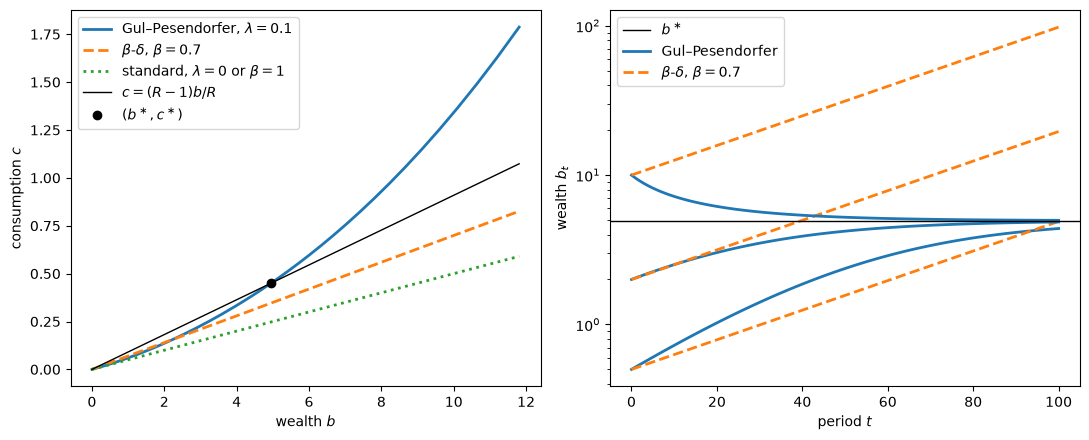
Fig. 75.1 Consumption rules and wealth paths#
In the left panel, the black line is the consumption \((R - 1) b / R\) that keeps wealth constant.
The Gul–Pesendorfer rule crosses it at the dot \((b^\ast, c^\ast)\): below \(b^\ast\) the consumer saves, and above \(b^\ast\) the consumer runs wealth down.
The \(\beta\)-\(\delta\) rule and the standard rule lie below the black line at every level of wealth, so those consumers accumulate wealth without bound.
In the right panel, wealth paths of the Gul–Pesendorfer consumer from three initial levels converge to \(b^\ast \approx 4.95\), while wealth paths of the \(\beta\)-\(\delta\) consumer grow at the constant gross rate \(R(1 - \kappa) \approx 1.023\).
75.4.3. Self-control as a property of preferences#
Gul and Pesendorfer contrast the two approaches in their conclusion.
In the \(\beta\)-\(\delta\) approach, a decision problem may not have a unique payoff, because the game among selves can have many subgame-perfect equilibria.
They argue that multiplicity is hard to interpret in a problem with a single decision maker:
In that case, the game-theoretic argument for multiplicity loses much of its force since it should be straightforward to renegotiate one’s self out of an unattractive continuation equilibrium.
They attribute the argument about renegotiation to Kocherlakota [1996].
Gul and Pesendorfer argue that the \(\beta\)-\(\delta\) approach can model self-control only by selecting an equilibrium in which the threat of worse behavior after a deviation sustains good behavior, so that self-control is a property of the selected equilibrium.
In the Gul–Pesendorfer approach, each \((u, v, \delta)\) represents a unique preference, all optimal plans yield the same payoff, and self-control is a property of the preference, measured by parameters such as \(\lambda\).
75.5. Equilibrium implications#
75.5.1. Steady-state wealth distributions#
Gul and Pesendorfer study an exchange economy with one good, a constant aggregate endowment \(\omega\), and consumers \(i = 1, \ldots, n\) who share \(u\), \(v\), and \(\delta\) but differ in self-control: consumer \(i\) has temptation utility \(\lambda_i v\).
Their Proposition 2 states that each aggregate endowment has a unique steady-state equilibrium, in which a consumer with more self-control consumes more.
With \(u(c) = \log c\) and \(v(c) = c\), the Euler equation (75.9) in a steady state with gross interest rate \(R\) becomes \(1 + \lambda_i c_i = \delta R\).
Writing \(\gamma_i = 1 / \lambda_i\) and imposing \(\sum_i c_i = \omega\) gives
The steady-state distribution of consumption and wealth depends on the \(\lambda_i\) and on \(\omega\), and not on the initial distribution of wealth.
A mean-preserving spread of the \(\gamma_i\) raises inequality and leaves \(R\) unchanged, while a larger \(\omega\) raises \(R\) and leaves consumption shares unchanged.
When every \(\lambda_i = 0\), the steady state requires \(\delta R = 1\), and any division of the aggregate endowment among consumers is a steady state.
The next cell computes (75.13) for three consumers with \(\lambda_i = 0.05\), \(0.1\), and \(0.2\), \(\omega = 3\), and \(\delta = 0.95\), and checks it against the consumer’s problem.
It solves each consumer’s problem (75.8) at the steady-state interest rate and simulates from equal initial wealth.
def steady_state(λ_list, ω, δ):
    "Steady-state consumption of each consumer and the gross interest rate."
    γ = 1 / np.asarray(λ_list)
    return ω * γ / γ.sum(), (ω + γ.sum()) / (δ * γ.sum())

λ_list, ω = (0.05, 0.1, 0.2), 3.0
c_ss, R_ss = steady_state(λ_list, ω, δ=0.95)
b_ss = R_ss * c_ss / (R_ss - 1)
print(f"steady-state gross interest rate R = {R_ss:.4f}")

b_0 = b_ss.mean()
for λ_i, c_i, b_i in zip(λ_list, c_ss, b_ss):
    con_i = create_consumer(δ=0.95, R=R_ss, λ=λ_i)
    _, c_i_grid = solve_consumer(con_i)
    b_path, c_path = simulate(c_i_grid, con_i, b_0, periods=300)
    print(f"λ = {λ_i}: steady state c = {c_i:.4f}, b = {b_i:.4f}; "
          f"from b_0 = {b_0:.2f}, c_300 = {c_path[-1]:.4f}, "
          f"b_300 = {b_path[-1]:.4f}")
steady-state gross interest rate R = 1.1429
λ = 0.05: steady state c = 1.7143, b = 13.7143; from b_0 = 8.00, c_300 = 1.7143, b_300 = 13.7143
λ = 0.1: steady state c = 0.8571, b = 6.8571; from b_0 = 8.00, c_300 = 0.8571, b_300 = 6.8571
λ = 0.2: steady state c = 0.4286, b = 3.4286; from b_0 = 8.00, c_300 = 0.4286, b_300 = 3.4286
At the steady-state interest rate, each consumer’s wealth converges from the common initial level to \(b_i = R c_i / (R - 1)\).
This is a partial-equilibrium check: along the transition, aggregate consumption differs from \(\omega\), so the constant interest rate \(R\) does not clear markets, and Gul and Pesendorfer do not study convergence to the steady state.
Steady-state wealth is inversely proportional to \(\lambda_i\): the consumer with \(\lambda_i = 0.05\) holds four times the wealth of the consumer with \(\lambda_i = 0.2\).
When \(v\) is strictly convex, the marginal rate of substitution between consumption at \(t\) and \(t + 1\) depends on wealth at \(t + 1\), through the term \(v'(b_{t+1})\) in (75.9).
With the linear \(v\) of the example, that term is the constant \(\lambda\), and the Euler equation can be written \(1/c_t = [\delta/(1 + \lambda c_t)] \, R / c_{t+1}\): the consumer acts as if its discount factor \(\delta/(1 + \lambda c_t)\) falls as its consumption rises.
Gul and Pesendorfer compare this feature with the endogenous rates of time preference of Uzawa [1968] and Epstein and Hynes [1983], in which the marginal rate of substitution depends on later consumption and therefore on wealth.
75.5.2. Inefficiency and nonbinding constraints#
A consumer’s welfare depends on the set of consumption bundles that it can afford at given prices and wealth, not only on the bundle that it chooses.
Gul and Pesendorfer therefore define Pareto efficiency for a planner who can reallocate resources and change prices but cannot remove options from consumers’ budget sets.
They give an example of a two-good economy with a representative consumer in which, they argue, the planner raises welfare by destroying some of the endowment of the tempting good.
Destroying the good raises its price, which lowers the amount of it that the consumer can afford and so lowers the cost of self-control.
Gul and Pesendorfer argue that in their example this effect outweighs the loss of consumption, and that a tax on the tempting good has the same effect if the government uses the proceeds to buy and destroy the good.
Their calculation uses equilibrium prices that omit the self-control term of the Euler equation (75.9).
With prices that satisfy (75.9), destroying the tempting good lowers welfare in their example for every \(\lambda \in (0, 1/2)\), so the example does not establish their claim.[1]
They also show that adding a borrowing constraint that does not bind in equilibrium changes equilibrium prices.
In their example, the constraint limits each consumer’s borrowing to its endowment in the next period.
The constraint lowers the maximal consumption available to the consumer in each period, and with it the cost of self-control.
To keep the Euler equation (75.9) satisfied, the equilibrium interest rate falls.
Consumption then tracks income: consumers do not shift funds to low-income periods, because doing so would raise the maximal consumption available in those periods and with it the cost of self-control.
75.5.4. Sustainable debt#
Bulow and Rogoff [1989] show that if the only punishment for default is exclusion from future borrowing, and a defaulter can still save at the market interest rate, then a consumer with standard preferences cannot borrow at all.
A consumer who defaults and saves the amounts that it would have repaid can finance strictly more consumption than the contract provides, so it prefers to default.
Gul and Pesendorfer show that a consumer with dynamic self-control preferences can borrow under such a contract.
A debt contract extends credit that becomes available only at a later date, so the consumer does not bear the self-control cost of having the funds available in the meantime.
Savings, in contrast, remain available to consume, so they raise the cost of self-control.
Gul and Pesendorfer add that creditworthiness, unlike savings, cannot serve as collateral, so the consumer cannot undo the commitment of a debt contract in the market.
Their Proposition 3 gives a contract with a three-period cycle of borrowing and repayment that a consumer with a kinked commitment utility and linear temptation utility prefers to honor when \(\delta\) is close enough to one, the interest rate is at most \((1 - \delta)/\delta\), and its temptation parameter \(\lambda\) lies in an interval.
75.6. Connections to other lectures#
Time Inconsistency of Ramsey Plans defines dynamic programming squared, the structure of the \(\beta\)-\(\delta\) equilibrium (75.11)–(75.12).
Institution Building Without Commitment studies a planner with \(\beta\)-\(\delta\) preferences and compares Markov, Ramsey, and organizational equilibria of the game among successive selves.
Optimal Savings I: Cake Eating and Optimal Savings II: Numerical Cake Eating solve a cake-eating problem, the case \(v = 0\) and \(R = 1\) of (75.8), by value function iteration.
Doubts or Variability? uses recursive preferences of the kind studied by Kreps and Porteus [1978], which allow the preference for early resolution of uncertainty that the Gul–Pesendorfer axiom of indifference to timing rules out.
75.7. Exercises#
Exercise 75.1
Kreps’s proof of his Theorem 1 constructs a state space and a utility function from a ranking of menus.
For a menu \(x\), define \(f(x)\) as the union of all menus \(x'\) with \(x \sim x \cup x'\); \(f(x)\) is the largest menu that contains \(x\) and is indifferent to \(x\).
The states are the menus \(s\) with \(f(s) = s\), and \(U(z, s) = 0\) if \(z \notin s\) and \(U(z, s) = a(s) < 0\) if \(z \in s\), so that
Kreps’s Lemma 3 chooses the negative numbers \(a(s)\) by induction, starting with the best states and moving down, so that each state’s sum \(\sum_{s' \supseteq s} a(s')\) is equal within a class of indifferent states and lower than the sums of all better states.
Let \(Z = \{\text{steak}, \text{chicken}, \text{fish}\}\), and generate a ranking of the seven menus from (75.3) with two moods: a hungry mood, with probability \(0.6\) and utilities \(3, 1, 0\) for steak, chicken, and fish, and a light mood, with probability \(0.4\) and utilities \(0, 2, 3\).
Solution
Z = ('steak', 'chicken', 'fish')
menus = [frozenset(c) for k in range(1, 4) for c in combinations(Z, k)]
moods = [(0.6, {'steak': 3, 'chicken': 1, 'fish': 0}),
         (0.4, {'steak': 0, 'chicken': 2, 'fish': 3})]
value = {x: round(sum(π * max(U[z] for z in x) for π, U in moods), 10)
         for x in menus}

def indifferent(x, y, value):
    "True if the ranking given by value is indifferent between x and y."
    return value[x] == value[y]

flexibility = all(value[x | y] >= value[x] for x in menus for y in menus)
property_15 = all(indifferent(x | w, x | y | w, value)
                  for x in menus for y in menus if indifferent(x, x | y, value)
                  for w in menus)
print(f"(tsc-flexibility) holds: {flexibility}; "
      f"(tsc-kreps-15) holds: {property_15}")

f = {x: frozenset().union(*[y for y in menus if indifferent(x, x | y, value)])
     for x in menus}
states = [x for x in menus if f[x] == x]

a, total = {}, {}             # total[s] is the sum of a(s') over s' ⊇ s
for level in sorted({value[s] for s in states}, reverse=True):
    group = [s for s in states if value[s] == level]
    partial = {s: sum(a[t] for t in a if t > s) for s in group}
    target = min(list(partial.values()) + list(total.values())) - 1.0
    for s in group:
        a[s], total[s] = target - partial[s], target

kreps = {x: sum(a[s] for s in states if s >= x) for x in menus}
same = all((value[x] >= value[y]) == (kreps[x] >= kreps[y])
           for x in menus for y in menus)
print(f"Kreps's representation reproduces the ranking: {same}")
print(f"number of states: {len(states)} (two moods generated the ranking)")
for x in sorted(menus, key=lambda x: -value[x]):
    print(f"{', '.join(sorted(x)):22s} two-mood value {value[x]:.2f}, "
          f"Kreps value {kreps[x]:5.1f}, f(x) = {', '.join(sorted(f[x]))}")
(tsc-flexibility) holds: True; (tsc-kreps-15) holds: True
Kreps's representation reproduces the ranking: True
number of states: 6 (two moods generated the ranking)
fish, steak            two-mood value 3.00, Kreps value  -1.0, f(x) = chicken, fish, steak
chicken, fish, steak   two-mood value 3.00, Kreps value  -1.0, f(x) = chicken, fish, steak
chicken, steak         two-mood value 2.60, Kreps value  -2.0, f(x) = chicken, steak
steak                  two-mood value 1.80, Kreps value  -3.0, f(x) = steak
chicken, fish          two-mood value 1.80, Kreps value  -3.0, f(x) = chicken, fish
chicken                two-mood value 1.40, Kreps value  -5.0, f(x) = chicken
fish                   two-mood value 1.20, Kreps value  -6.0, f(x) = fish
The two-mood ranking satisfies both properties.
The menu \(\{\text{steak}, \text{fish}\}\) is indifferent to \(Z\), because in each mood steak or fish is at least as good as chicken, so \(f(\{\text{steak}, \text{fish}\}) = Z\) and \(\{\text{steak}, \text{fish}\}\) is not a state.
Kreps’s construction uses six states, one for each menu with \(f(s) = s\), where two moods suffice.
Kreps notes that the construction uses many states and that other, smaller collections of states also represent the ranking; his Theorem 2 characterizes the collections that represent it in the ordinal form of his Theorem 1′, and he notes that not every such collection admits the additive form (75.3).
Exercise 75.2
Consider the preference reversal experiment of the lecture, with baseline consumption \(\bar c = 1\), \(u(c) = \log c\), and \(\delta = 0.95\).
A Gul–Pesendorfer consumer has \(v(c) = \lambda c\) with \(\lambda = 0.2\).
A \(\beta\)-\(\delta\) consumer has \(\beta = 0.8\).
Show that the \(\beta\)-\(\delta\) consumer reverses its choice between the smaller reward \(m\) at date \(t\) and the larger reward \(M\) at date \(t + 1\) when \(\beta \delta D_M < D_m < \delta D_M\).
For \(m \in (0, 2]\), compute and plot the smallest and largest \(M\) that produce a reversal for each consumer, and the width of the range of \(D_M\) that produces a reversal.
How does the range of \(M\) that produces a reversal depend on \(m\) in the two models?
Solution
A \(\beta\)-\(\delta\) consumer who decides at date \(t\) compares \(u(\bar c + m) + \beta \delta u(\bar c)\) with \(u(\bar c) + \beta \delta u(\bar c + M)\) and takes the smaller reward if \(D_m > \beta \delta D_M\).
A \(\beta\)-\(\delta\) consumer who decides at date \(t - 1\) compares \(\beta \delta u(\bar c + m) + \beta \delta^2 u(\bar c)\) with \(\beta \delta u(\bar c) + \beta \delta^2 u(\bar c + M)\) and takes the smaller reward if \(D_m > \delta D_M\).
The consumer reverses its choice when \(\beta \delta D_M < D_m < \delta D_M\).
With \(u(c) = \log c\) and \(\bar c = 1\), \(D_\rho = \log(1 + \rho)\), so each condition on \(D_M\) gives a bound on \(M\) in closed form.
Both consumers prefer \(M\) when deciding in advance if \(\log(1 + M) > \log(1 + m)/\delta\).
The Gul–Pesendorfer consumer takes \(m\) when deciding at date \(t\) if \(\log(1 + M) < [\log(1 + m) + \lambda m]/\delta\), and the \(\beta\)-\(\delta\) consumer if \(\log(1 + M) < \log(1 + m)/(\beta \delta)\).
δ_ex, λ_ex, β_ex = 0.95, 0.2, 0.8           # parameters of the exercise
m = np.linspace(0.005, 2, 400)
D_m = np.log(1 + m)
M_low = np.exp(D_m / δ_ex) - 1                      # both consumers
M_high_gp = np.exp((D_m + λ_ex * m) / δ_ex) - 1     # Gul–Pesendorfer
M_high_βδ = np.exp(D_m / (β_ex * δ_ex)) - 1         # β-δ

fig, axes = plt.subplots(1, 2, figsize=(11, 4.5))
ax = axes[0]
ax.plot(m, M_low, 'k', lw=1, label='lower bound, both models')
ax.plot(m, M_high_gp, 'C0', lw=2, label='upper bound, Gul–Pesendorfer')
ax.plot(m, M_high_βδ, 'C1--', lw=2, label=r'upper bound, $\beta$-$\delta$')
ax.set_ylabel('larger, later reward $M$')
ax = axes[1]
ax.plot(m, λ_ex * m / δ_ex, 'C0', lw=2,
        label=r'Gul–Pesendorfer, $S_m / \delta$')
ax.plot(m, (1 - β_ex) * D_m / (β_ex * δ_ex), 'C1--', lw=2,
        label=r'$\beta$-$\delta$, $(1 - \beta) D_m / (\beta \delta)$')
ax.set_ylabel('width of the reversal range of $D_M$')
for ax in axes:
    ax.set_xlabel('smaller, earlier reward $m$')
    ax.legend()
plt.tight_layout()
plt.show()

cross = m[np.argmax(M_high_gp > M_high_βδ)]
print(f"the Gul–Pesendorfer upper bound exceeds the β-δ upper bound "
      f"for m > {cross:.2f}")
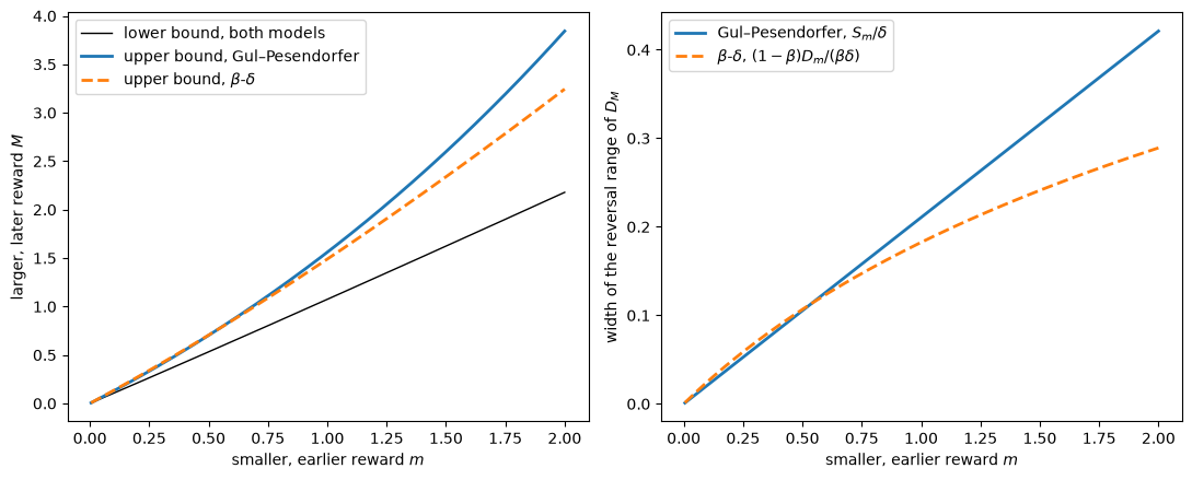
the Gul–Pesendorfer upper bound exceeds the β-δ upper bound for m > 0.54
In both models, the consumer reverses its choice when \(M\) is large enough that the consumer prefers it when deciding in advance, \(\delta D_M > D_m\), but not so large that the consumer takes it when deciding at date \(t\).
In the \(\beta\)-\(\delta\) model, the upper bound on \(D_M\) is \(D_m / (\beta \delta)\), a multiple of \(D_m\), so the range of reversals in terms of utility gains is proportional to the utility gain of the smaller reward.
In the Gul–Pesendorfer model, the upper bound on \(D_M\) is \((D_m + S_m)/\delta\), so the range is proportional to the self-control cost \(S_m = \lambda m\), which grows linearly in \(m\) while \(D_m = \log(1 + m)\) grows more slowly.
With these parameters, the Gul–Pesendorfer consumer reverses for a wider range of \(M\) when \(m\) exceeds about \(0.54\), and the \(\beta\)-\(\delta\) consumer for a wider range when \(m\) is smaller.
Exercise 75.3
In the Lucas tree economy of Gul and Pesendorfer, a representative consumer owns one share of a tree whose dividend \(d\) is independently and identically distributed over time with mean \(1\), variance \(\sigma^2\), and support \([0, 2]\).
The consumer has the commitment and temptation utilities of the lecture, with \(0 < \lambda < 1/2\).
In equilibrium the consumer consumes the dividend, and the price \(p\) of the tree is constant.
Use the Euler equation for the tree, \(p \, [u'(c_t) + v'(c_t)] = \delta E \{ [u'(c_{t+1}) + v'(c_{t+1}) - v'(p + d_{t+1})] (p + d_{t+1}) \}\), to show that \(p = \delta [1 + p - 2 \lambda p - \lambda p^2 - \lambda(\sigma^2 + 1)]\).
Show that the gross risk-free rate satisfies \(1/(1 + r^f) = \delta [1 - \lambda (p + 1)]\).
Let \(1 + r^e = (1 + p)/p\) be the expected gross return on the tree, and let \(d\) be uniformly distributed on \([0, 2]\) and \(\delta = 0.95\); compute \(p\), \(r^f\), and \(r^e - r^f\) for \(\lambda \in (0, 0.1]\), and check Gul and Pesendorfer’s formula \(r^e - r^f = \lambda \delta \sigma^2 (1 + r^f)/p\).
Check the Euler equation for the tree by numerical integration over \(d\).
Solution
With \(u(c) + v(c) = c\), marginal utility \(u' + v'\) equals \(1\), and \(v'(p + d) = \lambda (p + d)\).
The Euler equation for the tree becomes \(p = \delta E[(1 - \lambda (p + d))(p + d)] = \delta [p + 1 - \lambda E(p + d)^2]\).
Since \(E(p + d)^2 = p^2 + 2p + \sigma^2 + 1\), this is the equation in part 1.
A risk-free bond that pays one unit next period satisfies \(1/(1 + r^f) = \delta E[1 - \lambda (p + d)] = \delta [1 - \lambda (p + 1)]\).
The equation for \(p\) is a quadratic with the positive root
def tree_prices(λ, δ, σ2):
    "Price of the tree, risk-free rate, and expected return on the tree."
    p = (np.sqrt((1 - δ)**2 + 4 * δ * λ * (1 - δ * λ * σ2))
         - (1 - δ + 2 * δ * λ)) / (2 * δ * λ)
    r_f = 1 / (δ * (1 - λ * (p + 1))) - 1
    r_e = (1 + p) / p - 1
    return p, r_f, r_e

δ_tree, σ2 = 0.95, 1 / 3                   # d uniform on [0, 2]
λ_grid = np.linspace(0.002, 0.1, 50)
p, r_f, r_e = tree_prices(λ_grid, δ_tree, σ2)
formula = λ_grid * δ_tree * σ2 * (1 + r_f) / p
print(f"largest gap between r_e - r_f and the formula: "
      f"{np.max(np.abs(r_e - r_f - formula)):.1e}")

d = np.linspace(0, 2, 200_001)             # quadrature nodes for d
for λ_i in (0.02, 0.05, 0.1):
    p_i, _, _ = tree_prices(λ_i, δ_tree, σ2)
    residual = p_i - δ_tree * np.mean((1 - λ_i * (p_i + d)) * (p_i + d))
    print(f"λ = {λ_i}: p = {p_i:.4f}, Euler equation residual = {residual:.1e}")

fig, axes = plt.subplots(1, 2, figsize=(11, 4.5))
axes[0].plot(λ_grid, 100 * r_f, lw=2, label='risk-free rate $r^f$')
axes[0].plot(λ_grid, 100 * r_e, lw=2, label='expected return on the tree $r^e$')
axes[0].set_ylabel('percent')
axes[0].legend()
axes[1].plot(λ_grid, 100 * (r_e - r_f), lw=2)
axes[1].set_ylabel('equity premium $r^e - r^f$ (percent)')
for ax in axes:
    ax.set_xlabel(r'$\lambda$')
plt.tight_layout()
plt.show()
largest gap between r_e - r_f and the formula: 4.9e-16
λ = 0.02: p = 5.0347, Euler equation residual = 6.3e-08
λ = 0.05: p = 3.0559, Euler equation residual = 1.6e-07
λ = 0.1: p = 1.9403, Euler equation residual = 3.2e-07
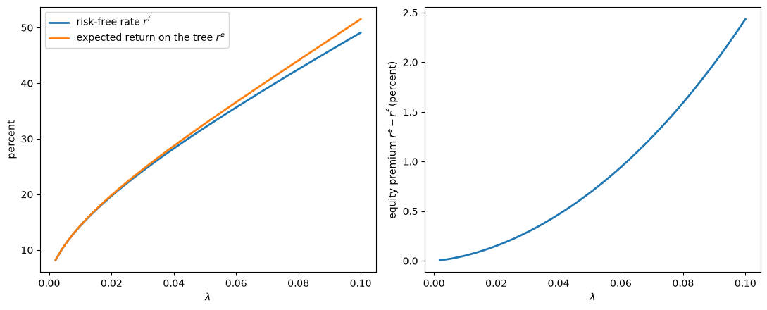
The premium is zero at \(\lambda = 0\), where the consumer is risk neutral, and rises with \(\lambda\).
Both rates of return rise steeply with \(\lambda\).
The price of the tree is large relative to its dividend, so the wealth \(p + d\) that tempts the consumer is large, and a small \(\lambda\) already makes the marginal self-control cost \(\lambda (p + d)\) of carrying wealth substantial.
With \(\delta = 0.95\), an equity premium of one percentage point requires \(\lambda \approx 0.062\), at which the risk-free rate is about \(36\) percent.